3 Vector data

Vector data was first used in CAD systems. They are suitable for measuring lengths, areas and for cartographic outputs on a pen plotter. Typical examples of this type of data are DXF, DWG (Autodesk), DGN (Intergraph), IGES (Initial Graphics Exchange Specification), HPGL (Hewlett Packard Graphic Language).

The vector expression of geographical phenomena captures objective reality more accurately than raster ones. The basis of vector data representation is the assumption that the space with mapped phenomena is continuous. Point phenomena are expressed by points, lines and areas are expressed only by means of representative points. Basic topological entities are expressed in vector format in the form of sequences of Cartesian x, y coordinates of their representative points. Due to the fine resolution of their coordinate system, they provide flexible and accurate representation of objects. Vector structures allow the interconnection of topology and other spatial connections between entities and phenomena and are therefore suitable for expressing complex spatial structures, such as networks (transport networks, river networks) or bodies.

The essence of vector data is the expression of the geometric part of the description of the geoelement using linear characteristics. The basic elements of vector data are:

• Point - expressed by a discrete position determined by x, y coordinates,
• Line - expressed by a sequence of oriented lines defined by the coordinates of their start and end point,
• Area - expressed by a closed contour line.

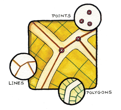
Figure 1: Vector data elements (source: https://saylordotorg.github.io/text_essentials-of-geographic-information-systems/s08-data-models-for-gis.html)

The basic spatial relationships between these elements were taken from graph theory. The graph consists of two parts - files: nodes and edges. Each edge is a connection of two nodes. If the order of the nodes is important when defining edges, it means that the edge has a direction. If the edges of the graph have a defined direction, the graph is oriented.

The direction of the edges and the subsequent orientation of the graph is important for several reasons. Oriented edges are a means of defining the orientation, direction of line objects, to describe the adjacency of the surfaces on the border - to the left and right of the edge. In addition, the direction is needed to describe the areas bounded by the lines of the planar graph.

Two edges are adjacent adjacent, if they have a common node. If there is a node in \(m\) edges, then the degree - order of this node is \(D (n) = m\). Therefore, if the order of the node \(D (n) = 0\), the node does not occur on any connector, it is an isolated node - a point.

A chain is a sequence of adjacent edges if it meets the following conditions:

• each edge occurs only once in a certain chain
• there are at most two nodes that occur on only one edge of the string. Their order is then \(D (n) = 1\) and they are the start and end node of the string.
• other nodes in the chain occur exactly in two edges, their order \(D (n) = 2\).

The closed string is called polygon, while there are no nodes in the polygon with the order \(D (n) = 1\), all have the order \(D (n) = 2\).

Two nodes in a graph are connected if there is a string in which both occur. A graph is connected if all possible nodel pairs are connected. By combining multiple polygons, we can build a network of polygons. When building it, we must pay attention to:

• non-duplicate designation of vertices and edges,
• inclusion of all necessary points and lines,
• distinguishing right and left areas for oriented maps,
• taking into account the “outdoor” area.

If such a structure consistently covers the entire examined area, it is called area partitioning. The so-called Euler’s equations can be used to check the completeness and uniqueness of the division of the surface, which follow the relationship between the number of nodes, edges and polygons. According to Euler’s rule, there is a fixed relationship between the number of facets \(f\), the number of nodes \(n\) and the number of edges \(e\) in the graph:

\(f+a-e=2\).

The rule in this basic form applies to connected graphs with surfaces without holes. For unlinked graphs it is necessary to modify it:

\(f+a-e=c+1\),

where \(c\) is the number of discontinuous subgraphs.

Based on the above, the basic building blocks for vector representation can perform different tasks in representing different types of objects:

• points - nodes who have two functions: your users as yours, resp. edge end nodes or intermediate points on lines (vertices) - in this case they are of exceptional importance for defining the geometry and topology of object lines, or representative bodies. Some bodily perform both functions at once. Points can appear in a representation that can only play in a geometric way, but do not represent point objects, nor are they nodes.
• edges - lines I can perform two functions: they can be representative of a line object or be part of a boundary between two planar objects.

It is not necessary to solve topological relations for the represented point objects. By specifying their position, we define their independence from other points. However, if the points fulfill the function of nodes, forming line objects, we must solve the affiliation of these nodes to individual lines.

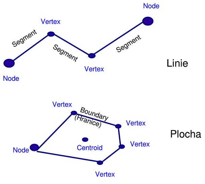
Figure 2: Vector data (source: http://les-ejk.cz/skoleni/grass/uvod/datove_typy/vektory.html)

If the represented line objects are connected, we must define their continuity at intersections - nodes. This relationship is called connectivity.

For represented planar objects we have to define three types of topological relations:

• continuity continuity of edges, forming the contour of a given surface in nodes - connectivity,
• affiliation of the edge to the given area, i.e. the relationship line - polygon or define areas (area definition),
• contiguity of surfaces - edges have a given direction, so we can determine the area to the right and left of the given edge, ie the continuity of surfaces - contiguity.

The position information is connected to the node or intermediate point (vertex) in the form of two of its attributes - coordinates \(x, y\). This method of localization is used for all types of objects, because their basic building blocks are points in all cases.

There are two basic approaches to modeling the thematic content (attributes) in vector representation - ways of organizing the database: layered and object-oriented.

Layered approach organization of the database with the creation of coverage - coverage is a classic approach, based on the design and creation of topographic and thematic maps in cartography. Coverage is a set of thematically related data considered as a unit. It usually represents an individual topic or information (e.g. soils, watercourses, unit settlements, etc.). Covers are organized so that they contain only geo-objects with the same geometric dimension and from one thematic class: point coverage - measuring points, dimensions, cities, wells, etc.; line coverage - watercourses, road network, product pipeline network, etc.; polygon coverage - plots, soil types, vegetation cover, etc.

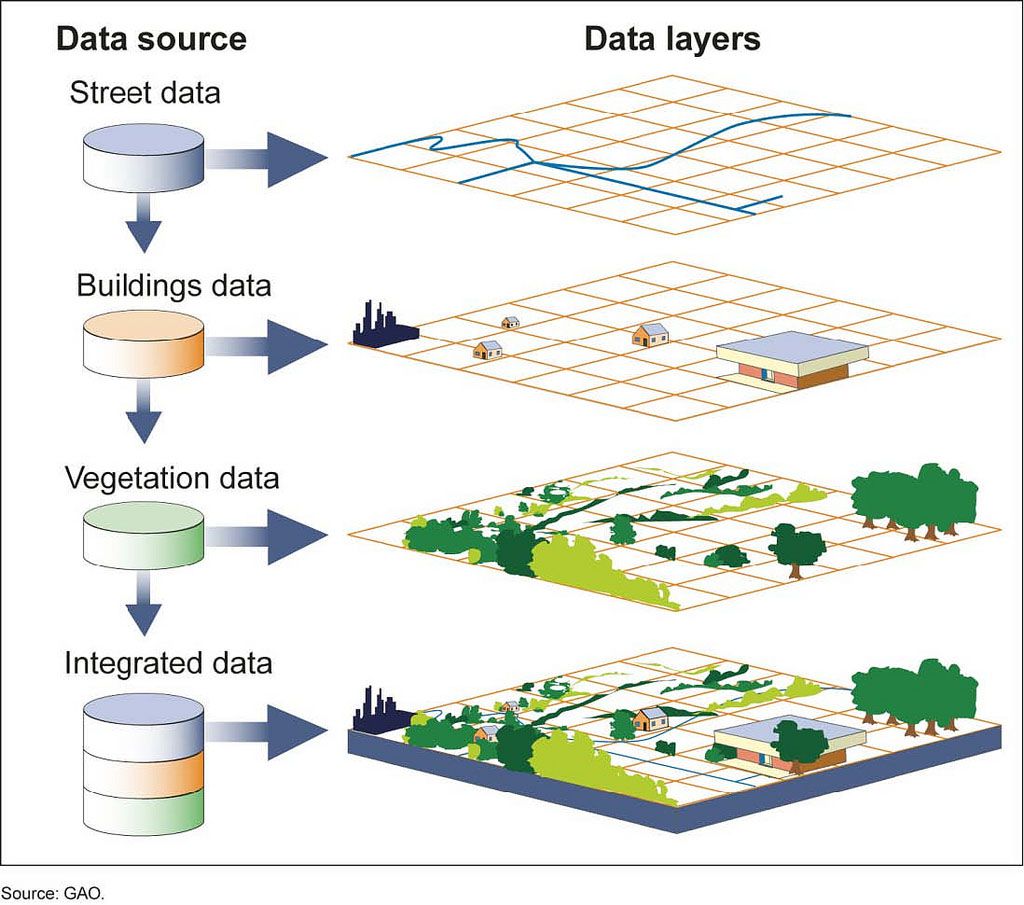
Figure 3: Vector layers (source: https://www.nationalgeographic.org/encyclopedia/geographic-information-system-gis/)

According to some authors, the advantages of the layered approach lie in:

• possibilities of creating thematic hierarchies,
• data acquisition, editing and access are handled specifically for each layer,
• very fast search by attribute.

The disadvantage is the more laborious and slower access to the object in terms of more (or all) attributes.

Object-oriented approach is newer, based on the principles of object-oriented data modeling. Its basic features are:

• each object has its own geometry, topology, theme and behavior,
• objects can be grouped into classes,
• it is possible to create hierarchical relationships between objects,
• attributes and methods are inherited by deriving for a subclass from an existing class.

Most usable vector data structures can be essentially classified into one of the following “classical types”:

• spaghetti model,
• topological model,
• hierarchical model.
  

3.1 Non-topological vector structures

3.1.1 Spaghetti model

Spaghetti model (unconnected vectors) is the simplest type. Each geofeature on the map is coded separately, without creating relationships with surrounding geofeatures. Basically, it is a direct transcription of the classic map line by line into digital form, so that a set of vectors and points in the form of X, Y coordinates is created without any information about interconnections (neighbor information is missing), lines can intersect practically arbitrarily. Today it is considered obsolete.

basic characteristics of the spaghetti model:

• neither the intersections of lines nor data on the logical interconnection of objects are marked,
• polygons - independent series of coordinates, the common boundary between two polygons is stored twice in the database, because each line is stored separately, often the coordinates of both variants of the common boundary are usually slightly different,
• when plotted, they create a tangle of intersecting lines - similar to “spaghetti”,
• most used for digitizing maps, where data is acquired by manual digitization or for digital photogrammetric registration, when it is necessary to reproduce the original image document,
• used mainly in computer graphics, digital cartography * spaghetti model is not suitable for spatial analysis, because any information about the relationships between objects, which is obvious when looking at the original analog document, must be derived by calculation,
• Storing and retrieving data - sequential - takes a long time.
  

3.2 Topological vector structures

3.2.1 Topological model

The basis of the topological model is the recording of the lines forming the map in the form of a planar graph.

Topology - the field of mathematics, which is called the description and analysis of spatial relationships between geometric objects. The topological model expresses the connections and bonds between objects independently of their coordinates - their topology remains unchanged even if they are stretched or bent. In GIS, it is mostly used for storing spatial data. Requires all lines to be continuous and polygons closed.

An edge begins and ends at the intersection with another edge, at the node. Each individual edge has a recorded designation and coordinates of its node points (beginning and end). It also records the identifier or name of the left and right adjacent polygons. In this way, spatial relationships are explicitly expressed and can be used in analyzes. This topological information allows to spatially define points, lines and areas and store them in a non-redundant way, which is especially advantageous for adjacent polygons, because each edge is stored only once, ie the common edge. Attributes are in separate relational tables; the topology is useful for rapid analysis of spatial functions without complex calculations using coordinates.

The problem with the spaghetti and topological model is that the individual records of the entities are not arranged in it. If we want to find a partial edge in the topological structure, we have to search the whole file sequentially. To find all the edges that define the boundary of a particular polygon, the search must be performed as many times as the edges make up that boundary.

Sometimes such an arrangement is also referred to as a NAA (Node-Arc-Area) representation (e.g., Worboys, 1995). The basic components of the model are: oriented arc - edge - arc, intersection - node - node and area - polygon - area. The system rules are as follows:

• Each oriented arc has one start and one end node.
• Each node must be the beginning or end of at least one arc.
• Each area is bounded by one or more oriented arcs.
• Oriented arcs can only intersect at their node points.
• Each oriented arc has exactly one area on the left and right.
• Each surface must be the right or left surface (or both) of at least one oriented arc.

The topological model is basically based on three basic topological rules:

1. Connectivity - describes the arc node topology for the function data set. As mentioned earlier, nodes are more than simple points. In a topological data model, nodes are intersections where two or more arcs meet. In the case of an arc node topology, arcs have both a node (i.e., the starting node) indicating where the arc begins and a node (i.e., the ending node) indicating where the arc ends (Figure 4). In addition, there is a line between each pair of nodes, sometimes called a connection, which has its own identification number and refers to both the node and the node. In Figure 5, arcs 1, 2 and 3 intersect because they share node 11. The computer can therefore determine that it is possible to move around arc 1 and turn to arc 3, while it is not possible to go from arc 1 to arc 5, because do not share a common node.

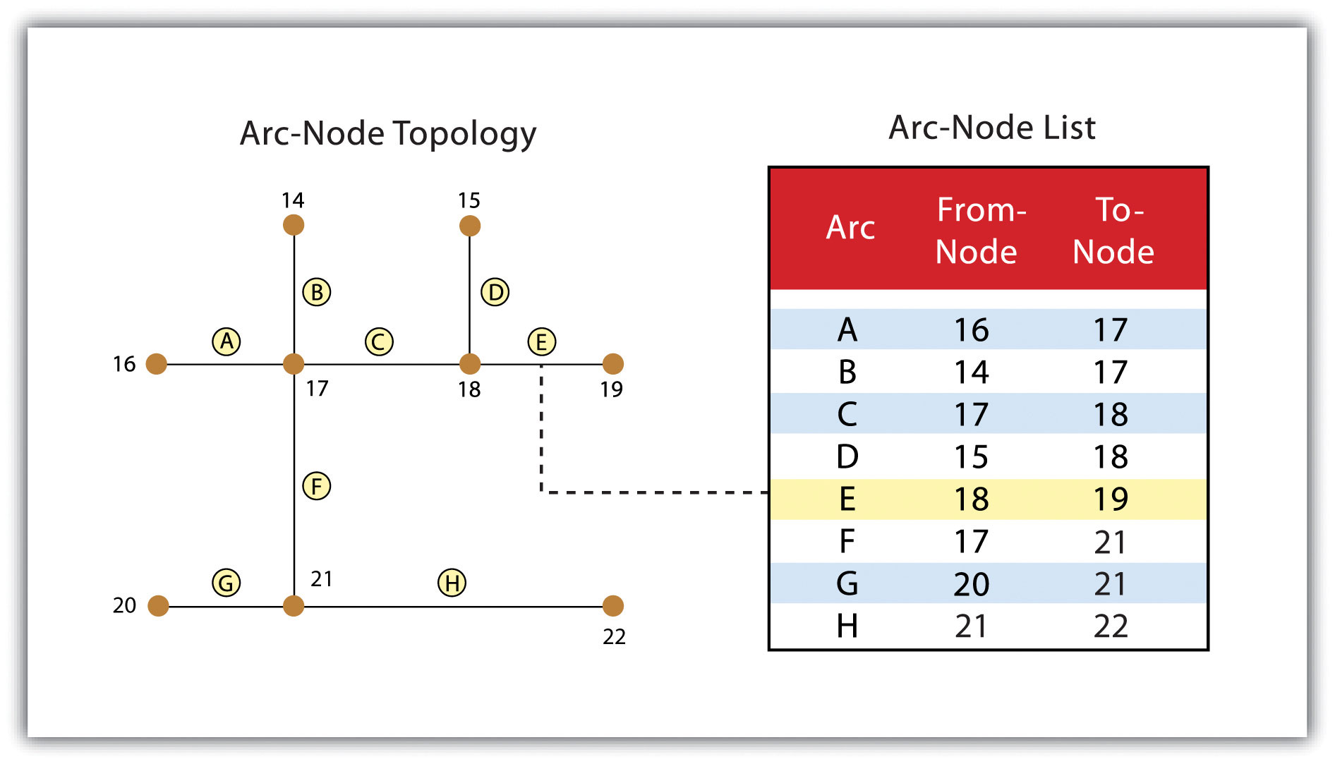
Figure 5: Topology arc - node (source: https://saylordotorg.github.io/text_essentials-of-geographic-information-systems/s08-data-models-for-gis.html)

2. Closedness (line) - the second basic topological regulation is the definition of the area. The area definition states that the arc that joins to surround the area defines a polygon, also called the polygon arc topology. In the case of a polygon arc topology, arcs are used to construct polygons, and each arc is stored only once (Figure 6). This reduces the amount of data stored and ensures that adjacent polygon boundaries do not overlap. It can be seen in Figure 6 that the polygon F is formed by arcs 8, 9 and 10.

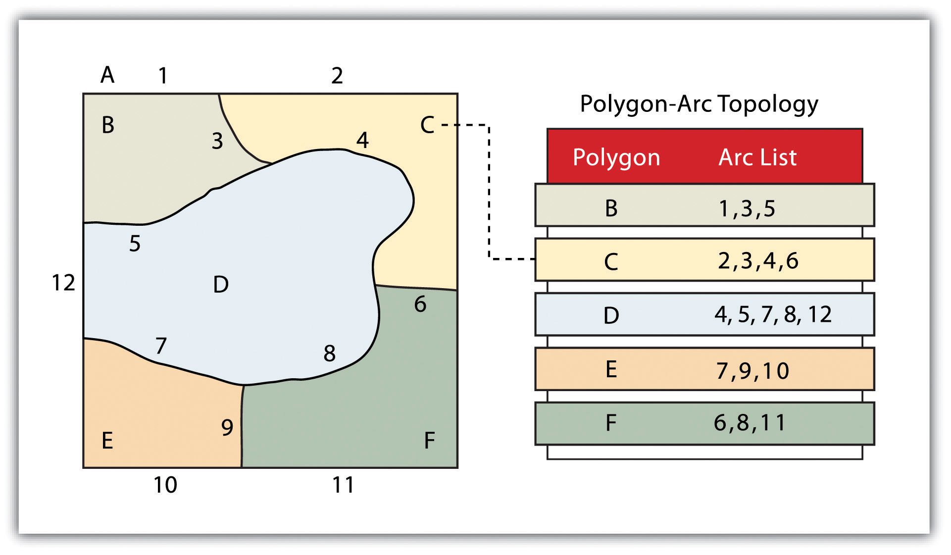
Figure 6: Topology arc - polygon (source: https://saylordotorg.github.io/text_essentials-of-geographic-information-systems/s08-data-models-for-gis.html)

3. Contiguity - is based on the concept that polygons that share a boundary are considered contiguous. Specifically, the topology of a polygon requires that all arcs in the polygon have a direction (from node to node), which allows you to determine neighborhood information (Figure 7). Polygons that share an arc are considered adjacent or contiguous, and therefore the “left” and “right” sides of each arc can be defined. This left and right polygon information is explicitly stored in the attribute information of the topological data model. The “space polygon” is an essential part of the polygon topology, which represents the outer area located outside the study area. Figure 7 shows that arc 6 is connected on the left by polygon B and on the right by polygon C. Polygon A, the polygon of space, is to the left of arcs 1, 2 and 3.

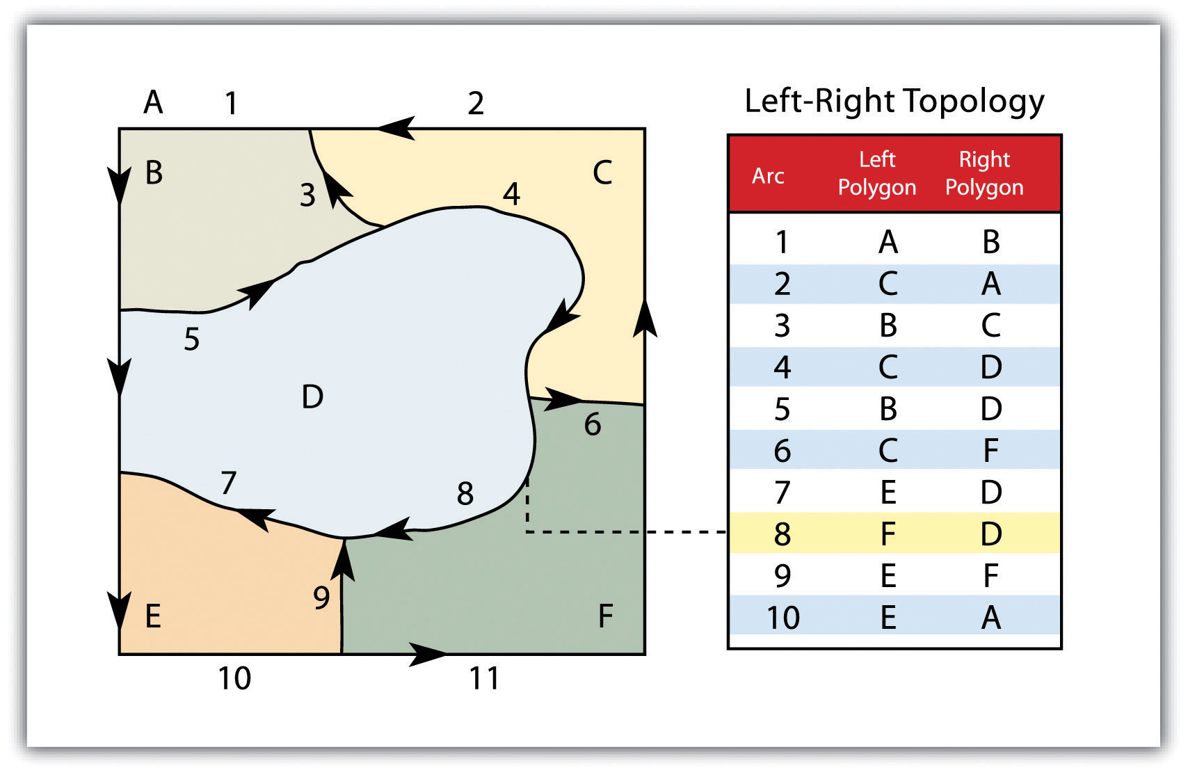
Figure 7: Polygon topology (source: https://saylordotorg.github.io/text_essentials-of-geographic-information-systems/s08-data-models-for-gis.html)

The topology allows the computer to quickly identify and analyze the spatial relationships of all its included functions. In addition, topological information is important because it enables efficient error detection within a vector data file. In the case of polygonal features, they break open or unclosed polygons that occur when the arc does not return completely, and unmarked polygons that appear when the area contains no attributes violate the rules of the polygon arc topology. Another topological error found in polygonal functions is the source. Fragments occur when the common boundary of two polygons is not exactly met (Figure 8).

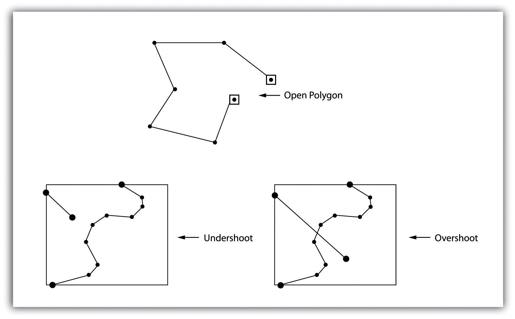
Figure 8: Common topological errors of vector data (source: https://saylordotorg.github.io/text_essentials-of-geographic-information-systems/s08-data-models-for-gis.html)

Many types of spatial analysis require a degree of organization offered by topologically explicit data models. In particular, network analysis (eg finding the best route from one place to another) and measurements (eg finding the length of a river section) strongly depend on the concept of nodes and edges, and uses this information together with attribute information to calculate distances, shortest routes, the fastest routes, etc. The topology also allows sophisticated neighborhood analysis, such as neighborhood determination, clustering, nearest neighbors, etc.

Such a topological model can be very conveniently represented in a relational database model.

3.2.2 Further improvement of the topological model

Double Connected Edge List

As an improvement to the NAA representation, Worboys (1995) cites the so-called DCEL (Double Connected Edge List) - a list of double-linked edges that improves the ability to search the structure by listing the previous and subsequent edges at each edge described.

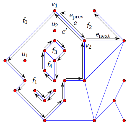
DCEL is more than just a double-linked list of edges. In the general case, the DCEL contains a record for each edge, vertex, and division area; each record can contain additional information, for example, a face can contain an area name. Each edge usually delimits two areas, so it is appropriate to consider each edge as two “half-edges” (which are shown on the right in Figure 8 by two edges in opposite directions, between two vertices); each “half edge” is “connected” to one surface and therefore has a pointer to that surface. All “half edges” associated with the surface are oriented clockwise or counterclockwise. For example, in the figure to the right, all “half-edges” associated with the center surface (ie, the “inner” half-edges) are counterclockwise. The half-edge has a pointer to the next half-edge and the previous half-edge of the same area. To reach the second surface, we can move to a pair of half-edges and then go through another surface; each half-edge also has a pointer to its initial vertex (the target vertex can be obtained by querying the origin of its twin or other half-edges).

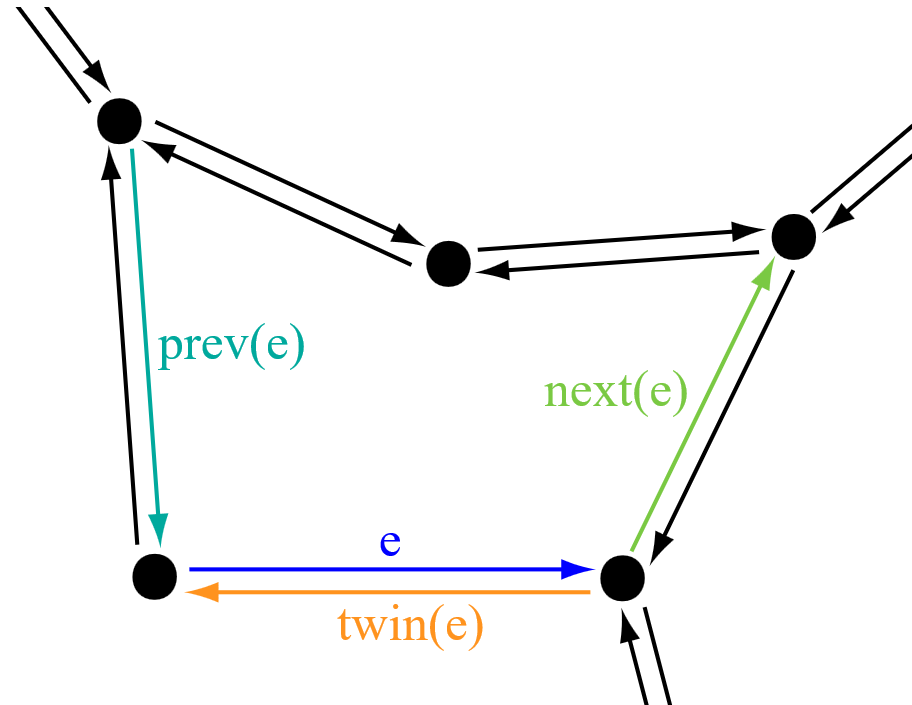
Figure 9: DCEL (source: https://wikivisually.com/wiki/Doubly_connected_edge_list)

DCEL is one of the combinatorial data structures, referred to as “half-edge data-structures”. Stores incidence relationships between 0-dimensional (vertices), 1-dimensional (edges), and 2-dimensional (areas) objects.

The DCEL structure thus consists of (see Figure 10):

• vertex - incident half-edge leading to this point
• halfedge * opposite half-edge * the previous half-edge in the boundary of the object * the next half-edge in the boundary of the object * target vertex hemispheres * incident area
• area - the incident half-edge of the area boundary
• interconnected part of the border * circular rectangular strings around surfaces

Windged Edge

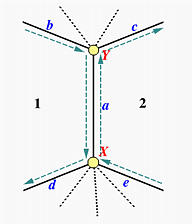
Edge (previous edge clockwise), na-edge (edge ​​following counterclockwise) Another improvement is the representation in the form of so-called winged edge - windged edge, which describes all possible information about the connections between nodes, edges and areas.

In the representation of a windged edge, the edge is considered to be the basic spatial object. Each edge is associated with its two respective surfaces: p-face, n-face and two vertices: p-vertex, n-vertex. Four additional edges are also tied to each edge, as indicated in Figure 11: nc-edge (clockwise edge), pc-left hand) and pa-edge (counterclockwise edge). This representation provides a complete characteristic of the topology in terms of incidence, adjacency and arrangement of edges, vertices and surfaces.

3.2.3 Hierarchical model

Hierarchical vector model overcomes the disadvantage of simpler vector models and structures when searching for entities by storing data on points, nodes, lines - edges and surfaces - polygons separately in a logical hierarchical structure. Polygons are defined by lines and these are represented as strings of points, ie. it is possible to explicitly build a connection model in which one type of object depends on another (see Figure 12). Such a link provides a direct search mechanism.

! [Figure 12: Hierarchical data model (source: Yuan, 2001)] (./ pictures / hierarchical_model.png)

Physical separation of individual classes of elements enables lower demands on memory space, speeding up most operations. On the contrary, this physical separation requires storing complex structures of search engines, identifiers. These non-data elements add a significant amount of required storage space and at the same time pose a potential problem in securing and maintaining data integrity.

3.3 Evaluation of vector data representation

Advantages

• it is possible to work with individual objects as separate units;
• less memory requirements;
• good representation of the phenomenal structure of data;
• High geometric accuracy
• quality graphics, accurate drawing, representation close to maps;
• Easy search, editing and generalization of objects and their attributes.
  

Disadvantages

• computational complexity (problems in complex analytical operations);
• complexity of the data structure;
• more complex answers to position questions;
• difficult overlay creation of vector layer overlays
• problems in modeling and simulation of phenomena.