9 Data sources for GIS III - Remote Sensing

Remote Sensing (RS) is a method of obtaining information about objects on the Earth’s surface without direct contact with it. Remote sensing includes the complete process of obtaining information from data acquisition, processing, analysis to the final visualization and interpretation of the image.

It is a modern geoinformation technology, which is currently becoming known to an ever-widening circle of professional and lay public. This is mainly due to the fact that this technology has a number of advantages over conventional ground measurements. The second reason is the constant development of satellite technologies and computer technology, and thus the simplification of previously demanding procedures.

Before studying this chapter, look at 100 Earth Shattering Remote Sensing Applications & Uses.

9.1 Basic principles of remote sensing

The basic principle of remote sensing is the measurement of the amount of electromagnetic radiation reflected or emitted by the earth’s surface (Figure 1). The source of this radiation is any object on the earth’s surface whose temperature is greater than absolute zero (i.e. -273.15 ° C). In the case of remote sensing, radiation emitted by the Earth’s surface itself is considered, as well as solar radiation reflected by the surface, or radiation emitted by an artificial source (e.g. radar) that reflects the Earth’s surface. The earth’s surface and the objects on it have certain physical properties; when electromagnetic radiation hits this surface, the radiation interacts with the specific surface on which it falls. The reflected radiation then gives us information about the surface from which it was reflected (Figure 2). Simply put, based on the radiation reflected by the earth’s surface, we are able to determine which substance it is.

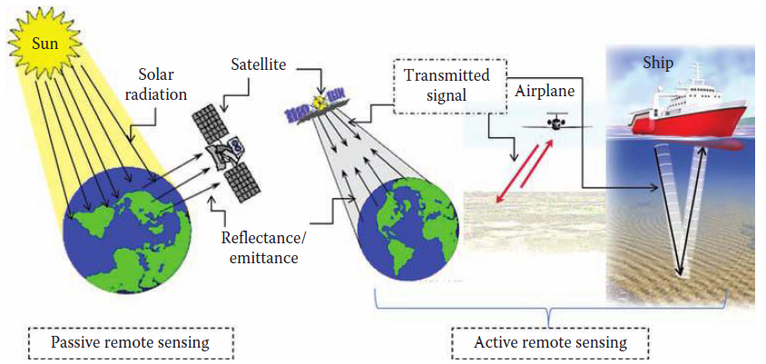
Figure 1: Illustration of passive vs. active remote sensing with different platforms. In passive remote sensing, the sun acts as the source of energy. Sensors then measure the reflected solar energy off the targets. Active remote sensing sends a pulse of synthetic energy and measures the energy reflected off the targets. (source: Thenkbail, 2016)

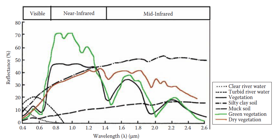
Figure 2: Typical reflectance curve of different objects generated with electromagnetic radiation frequency characteristics that are useful to distinguish/interpret objects (source: Thenkbail, 2016)

Electromagnetic radiation, which is reflected or emitted by the earth’s surface, is, in the case of remote sensing, recorded by special devices - radiometers, which can be carried by aircraft or satellites. Subsequently, we look for the relationship between the values of radiation measured by a radiometer and the properties of the earth’s surface, from which this radiation comes. The radiometer sensing electromagnetic radiation can be carried by satellite or aircraft, in rare cases ground carriers are also used.

Remote sensing has a number of advantages over conventional ground measurement methods. Data are acquired relatively quickly, even over large areas. At the same time, they are obtained for the entire area, thus eliminating the need for interpolation from point measurements. The measurements performed are repeatable; it is thus possible to obtain a time series of images for a certain period for a specific period. This also reduces the financial costs of data acquisition. At the same time, remote sensing enables the acquisition of information from hard-to-reach places. Thanks to the possibility of automating the entire process of processing satellite or aerial images, it is possible to better perform long-term and sustainable monitoring of the required area.

A great advantage of remote sensing is the ability to record information invisible to humans. The human eye is able to record only visible radiation with a wavelength range of approximately 380 - 720 nm (Figure 3), while for remote sensing, wavelengths of approximately 300 nm - 1 m are used.

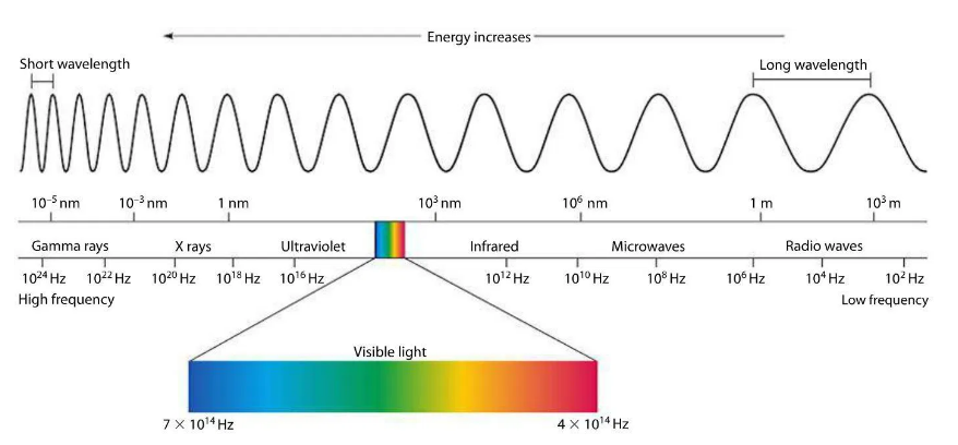
Figure 3: Electromagnetic spectrum (source: http://copernicus.gov.cz/zakladni-informace-a-princip-dpz)

When using longer wavelengths, it is possible to observe far more surface characteristics. E.g. vegetation has a much more pronounced effect in the infrared part of the spectrum than in the visible spectrum, making it far more distinguishable from other surfaces in infrared images. If the image was taken in the thermal part of the spectrum, it is possible to determine the temperature of objects on the earth’s surface from it.

Some satellites also have a so-called panchromatic band, which includes the area of visible radiation. This band tends to have a higher resolution than other bands; Using a technique called pansharpening, it is possible to improve the resolution of a multispectral image.

Remote sensing systems use two types of sensors (Figure 1) to sense (Bolstad, 2016):

passive - use energy generated by the sun and reflected off of the target objects. Aerial images and most satellite data are collected using passive systems. The images from these passive systems may be affected by atmospheric conditions in multiple ways. Figure 7 illustrates the many paths by which energy reaches a remote sensing device. Note that only one of the energy paths is useful, in that only the surface reflected energy provides information on the features of interest. The other paths result in no or only diffuse radiation reaching the sensor, and provide little information about the target objects. Most passive systems are not useful during cloudy or extremely hazy periods because nearly all the energy is scattered and no directly reflected energy may reach the sensor. Most passive systems rely on the sun’s energy, so they have limited use at night.
active - an alternative for gathering remotely sensed data under cloudy or nighttime conditions. Active systems generate an energy signal and detect the energy returned. Differences in the quantity and direction of the returned energy are used to identify the type and properties of features in an image. Radar (radio detection and ranging) is the most common active remote sensing system, while the use of LiDAR systems (light detection and ranging), is increasing. Radar focuses a beam of energy through an antenna, and then records the reflected energy. These signals are swept across the landscape, and the returns are assembled to produce a radar image. Because a given radar system is typically restricted to one wavelength, radar images are usually monochromatic (in shades of gray). These images may be collected day or night, and most radar systems penetrate clouds because water vapor does not absorb the relatively long radar wavelengths.

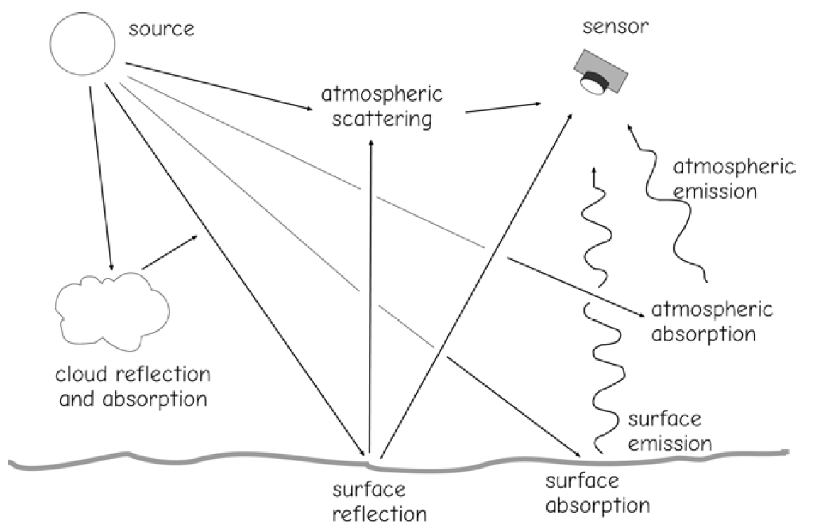
Figure 4: Energy pathways from source to sensor. Light and other electromagnetic energy may be absorbed, transmitted, or reflected by the atmosphere. Light reflected from the surface and transmitted to the sensor is used to create an image. The image may be degraded by atmospheric scattering due to water vapor, dust, smoke, and other constituents. Incoming or reflected energy may be scattered.(source: Bolstad, 2016)

In recent years, tremendous advancements in technology have resulted in a rapid growth in the remote sensing industry. During the last few decades, growth in the civilian sector has far surpassed the defense and military applications. However, the recent years have seen new applications of miniature remote sensors or camera systems that are mounted on both manned and unmanned aerial platforms, which are used by law enforcement and military sectors for surveillance purposes. Unmanned aerial vehicles (UAVs) are one of the most important advancements in aerial remote sensing in recent times and used even for fighting stealth wars. UAVs are now controlled from home base through onboard Global Positioning System (GPS) and forward-looking infrared (FLIR) and/or videography (FLIR) technology (Jensen, 2009). Other advances in remote sensing technology include RADAR, LiDAR, sound navigation and ranging (SONAR), sonic detection and ranging (SODAR), microwave synthetic aperture radar (SAR), infrared sensors, hyperspectral imaging, spectrometry, Doppler radar, and space probe sensors, in addition to improvements in conventional aerial photography, hyperspectral imaging, and imaging spectroradiometer (Thenkbail, 2016).

9.2 Photogrammetry

Photogrammetry deals with the reconstruction of shapes, measuring dimensions and determining the position of objects that are displayed in photographic images. More generally, photogrammetry can be defined as a discipline dealing with the processing of information in photographic images. Photogrammetry, for example, is an important part of Earth remote sensing (remote sensing). It is also used to evaluate meteor images taken by car cameras.

The name photogrammetry was formed by combining three Greek words photos - light, gramma - record, metron - measure. The word photogrammetry originated from an attempt to call a suitable term an activity dealing with the measurement of photographic images.

Photogrammetry is the art, science, and technique of obtaining information about physical objects and the environment through the process of recording, measuring, and interpreting photographic images and images of electromagnetic radiation patterns and other phenomena.

Information in photogrammetry can be imagined as geometric relationships, such as shape, size, position of displayed objects; when imaging in multiple spectral bands, the type and state of the object can also be determined. The advantage of photogrammetry is the use of a non-contact measurement method. Objects can be far from the shooting location.

9.2.1 Development of photogrammetry

The development of photogrammetry can be summarized in several milestones:

The origins go back well before the invention of photography (1839-Daguerre).
The first to put into practice central projection (basic imaging method in photogrammetry), Leonardo da Vinci (15th century) - using a pinhole camera (camera obscura) drew the central projections, from which he reconstructed map images.
The founder of photogrammetry is considered to be Laussedat (France), which began to use photographic images for measuring purposes.
The first photogrammetric measurement was performed by Dr. Loot - perforated he determined the location of important points in the territory of Prague (1867).
with the development of flying, aerial photogrammetry also began to develop - the first pictures from the air as early as 1858, but a great boom only during the first World War II (monitoring and interpretation purposes).
In the territory of our state is the first aerial stereophotogrammetric mapping took place in 1921.
Rapid development of computer technology in the late 80’s - the emergence of the first digital systems - a new area (digital photogrammetry).

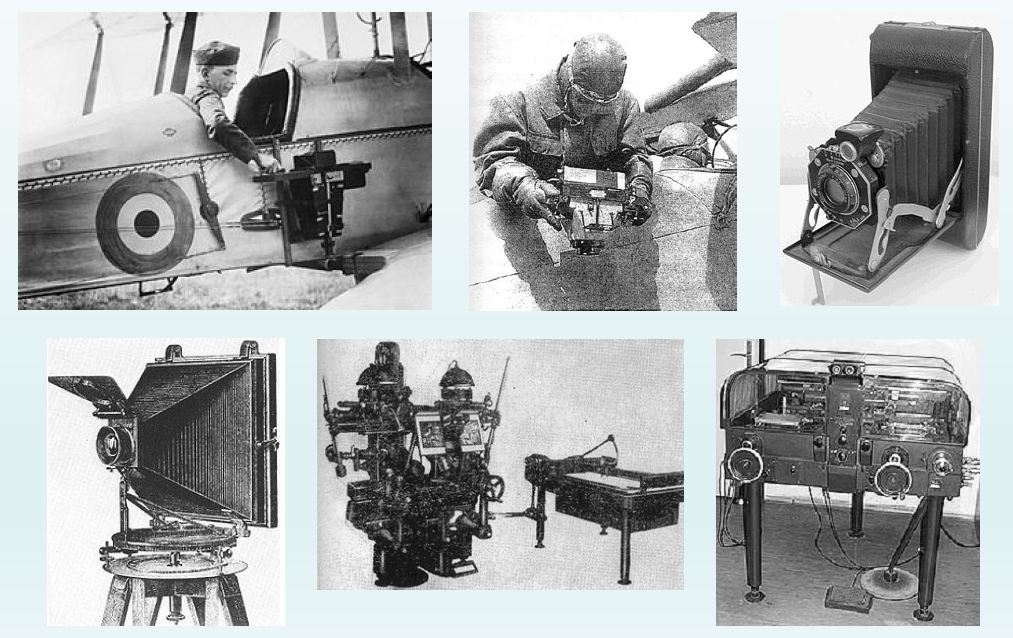
Figure 5: Snippets from the history of photogrammetry (source: http://uhulag.mendelu.cz/files/pagesdata/cz/geodezie/geodezie_2018/fotogrammetrie.pdf)

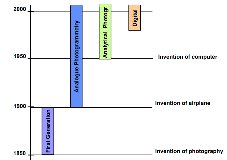
Figure 6: Different generations of photogrammetry (source: https://dprg.geomatics.ucalgary.ca/system/files/akam_431_ch_6_akam.pdf)

According to the number of evaluation images, we divide photogrammetry into:

single image - only planar coordinates can be measured on single images. In aerial photogrammetry, it is possible to obtain the topographical component of a flat area in this way, both from vertical and oblique images.
two-image - using two-image photogrammetry, the spatial coordinates of the object can be evaluated from a pair of images. The subject of the measurement must be displayed on both images at the same time. If stereoscopic perception is used to evaluate images, we speak of stereophotogrammetry.

According to the method of image processing (so-called conversion of image coordinates to planar or spatial coordinates), photogrammetry is divided into the method:

analogue - an optical-mechanical device operated by a specially trained operator with long-term training is required for evaluation.
analytical - the analytical method converts image coordinates into geodetic ones using spatial transformations, which are solved on computers.
digital - This method uses a digital image as input information. This can be a scanned classic image or an image taken directly with a digital camera.

The most commonly used types of outputs include:

3D point cloud,
orthophoto of the area of interest,
purpose map,
contour plan.

9.2.2 The principle of photogrammetry

Information about objects is not obtained by direct measurement, but by measurement their photographic images. Photogrammetry uses photographic images for its work, which are carriers of information (measuring, about objects of measurement-shape, size, position). the image is an exact central projection of the subject (an image of each point, line and plane is in turn a point, line and plane, object line and the pixel passes through the center of the projection). The basic task of photogrammetry is to convert this central projection into a rectangular projection. The input is a photographic image and the output is a map or plan. As part of the photo interpretation, we then recognize, identify and classify the objects displayed in the photographic images. The geometric relationships between the object and its image can be determined using photogrammetric instruments (numerically, graphically, mechanically).

We distinguish photogrammetry:

aerial:
terrestrial and
close.

Before imaging the surface, it is first necessary to perform photogrammetric signaling of points, at which it will then be geodetically measured. These points must contrast with the surroundings. There are 3 photogrammetric methods according to which imaging is performed: universal, combined and integrated.

9.2.3 Terrestrial photogrammetry

Because ground photogrammetry is most suitable for use at altitude rugged terrain, its field of application is very limited during mapping work. From the beginning, it was used mainly for mapping in alpine terrain. It is much more important in determining the volume of mining (even today) in surface mines, measuring the movements of bridges and dam bodies and to a large extent in construction when documenting facades, vaults and historic or otherwise important buildings. It is also used in criminology to document the location of a crime or traffic accidents, where it is known as oblique photogrammetry.

In construction, ground photogrammetry is used primarily for documentation buildings, whether monuments or new ones. It can be used for both exterior and interior targeting. Documentation of the condition of vaults, which would otherwise be difficult to focus on, is very quick and easy with the help of ground photogrammetry. Single-image photogrammetry is used for planar buildings, stereophotogrammetry for documentation of spatially divided structures. Figures 7 and 8 show an example of the use of classical terrestrial photogrammetry and its digital evaluation.

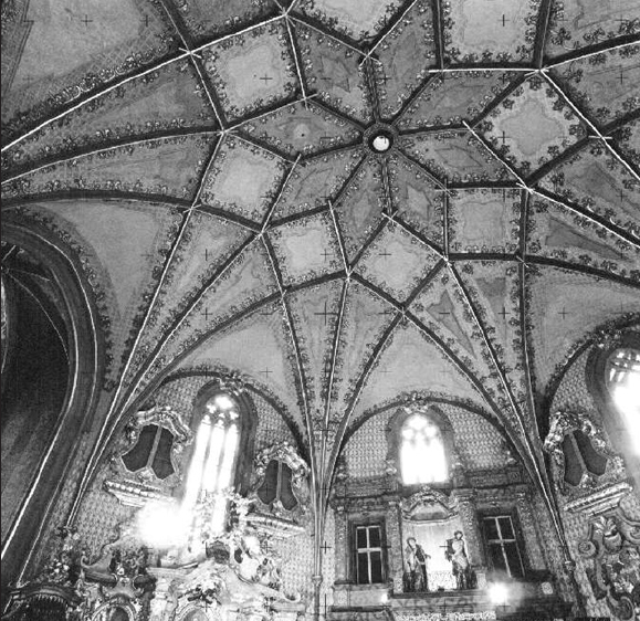
Figure 7: Photo of the arch of the church (zdroj: Böhm, 2002)

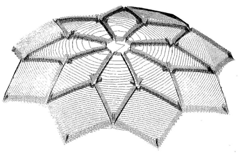
Figure 8: Contour plan of the vault - isometric view (zdroj: Böhm,2002)

More about terrestrial photogrammetry

9.2.4 Aerial photogrammetry

Aircraft are an older type of carrier. Images taken in this way usually have a better spatial resolution than in the case of satellite images. Their operation is more operative, ie. the aircraft can be directed faster over the scanned area than the satellite. The disadvantage of aircraft carriers is, in particular, greater spatial distortion and more expensive image acquisition than in the case of a satellite. Aerial images are used mainly for the creation of orthophotomaps (e.g. Orthophoto of the Czech Republic taken by ČÚZK). Due to the higher technological complexity of the construction of hyperspectral sensors, aircraft carriers are very often used for the acquisition of hyperspectral data. Examples are AISA or HyMap sensors, used mainly in the field of geology and for the study of vegetation.

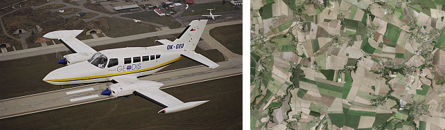
Figure 9: Aerial data (source: http://copernicus.gov.cz/zakladni-informace-a-princip-dpz)

Photogrammetry, the science of measuring geometry from images, was well developed by the early 1930s, and there have been continuous refinements since. Aerial images underpin most large-area maps and surveys in most countries. Digital mapping cameras have been become common in the 21st century, largely supplanting aerial cameras. Aerial images are routinely used in urban planning and management, construction, engineering, agriculture, forestry, wildlife management, and other mapping applications. Figure 10 shows the development in the quality of aerial photographs in time.

Figure 10: Improvement of the quality of aerial photogrammetry in time (source: https://www.slideshare.net/gokulsaud/photogrammetry-nec-for-students)

Although there are hundreds of applications for aerial images, most applications in support of GIS may be placed into three main categories. First, aerial images are often used as a basis for mapping, to measure and identify the horizontal and vertical locations of objects. Measurements on images offer a rapid and accurate way to obtain geographic coordinates, particularly when image measurements are combined with ground surveys. In a second major application, image interpretation may be used to categorize or assign attributes to surface features. For example, images are often used as the basis for landcover and infrastructure mapping, and to assess the extent of fire, flood, or other damage. Finally, images are often used as a backdrop for maps of other features, as when photographs are used as a background layer for soil survey maps produced by the U.S. National Resource Conservation Service.

Aerial photogrammetry is a geodetic method in which the geometric shape of a part of the earth’s surface is not determined in the field, but in its image taken from the air. A scanning device mounted on a flying carrier takes pictures during the flight. The ability of a photographic image - to capture a whole area of interest in a fraction of a second - is irreplaceable in documenting rapidly changing events, such as documenting areas affected by floods, storms, fires and the like. Its irreplaceability is in hard-to-reach or inaccessible areas, where another measuring method cannot even be used.

The advantage of aerial photogrammetry is therefore the large area shown in the image. The disadvantage is the ignorance of the exact spatial position of the image at the time of exposure, which leads to more complex processing. According to the direction of photography (direction of the axis of the shot) we recognize images (figure 12):

horizontal,
vertical,
oblique.

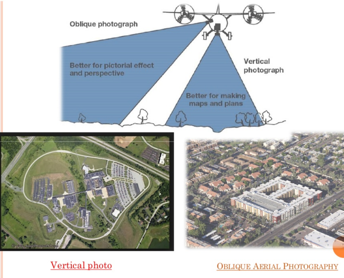
Figure 11: Vertical and oblique aerial photos (source: https://www.slideshare.net/gokulsaud/photogrammetry-nec-for-students)

According to the method of photography, we then distinguish the images:

individual (indicative),
in-line - photographed one after the other so that they overlap.

9.2.4.1 Camera Aircraft, Formats and Systems

Aerial camera systems are most often specifically designed for mapping, so the camera and components are built to minimize geometric distortion and maximize image quality. Mapping cameras have features to reduce image blur due to aircraft motion, enhancing image quality. They maintain or record orientation angles, so distortions can be minimized. These camera systems are precisely made, sophisticated, highly specialized, and expensive, and images suitable for accurate mapping are rarely collected with nonmapping cameras.

Mapping cameras are usually carried aboard specialized aircraft designed for photographic mapping projects. These aircraft typically have an instrument bay or hole cut in the floor, through which the camera is mounted. The camera mount and aircraft control systems are designed to maintain the camera optical axis as near vertical as possible. Aircraft navigation and control systems are specialized to support aerial photography, with precise positioning and flight control.

Aerial cameras for spatial data collection are large, expensive, sophisticated devices, but in principle they are similar to simple cameras. A simple camera consists of a lens and a body (Figure 17). The lens is typically made of several individual glass elements, with a diaphragm or other mechanism to control the amount of light reaching the sensing media, the digital sensor or film that records light. These sensors have a characteristic dimension, sd, and for digital sensors, a pixel size, that when combined with the flying height ($H$), and focal length ($h$), determine the ground resolution and imaged area. An exposure control, such as a shutter within the lens, controls the length of time the film is exposed to light. Cameras also have an optical axis, defined by the lens and lens mount. The optical axis is the central direction of the incoming image, and it is precisely oriented to intersect the sensor in a perpendicular direction. Digital sensors are connected to electronic storage, so that successive images may be saved, while film is typically wound on a supply reel (unexposed film) and a take-up reel (exposed film). Images are recorded on a flat stage called the camera’s focal plane, perpendicular to the optical axis. The time, altitude, and other conditions or information regarding the photographs or mapping project may be recorded by the camera, often as an electronic header on digital image files, or on the data strip for film cameras, a line of text in the margin of the photograph.

Image scale and extent are important attributes of remotely sensed data. Image scale, as in map scale, is defined as the relative distance on the image to the corresponding distance on the ground. For example, 1 inch on a 1:15,840-scale photograph corresponds to 15,840 inches on the Earth’s surface.As shown in Figure 12, image scale will be $h/H$, the ratio of focal length to flying height.

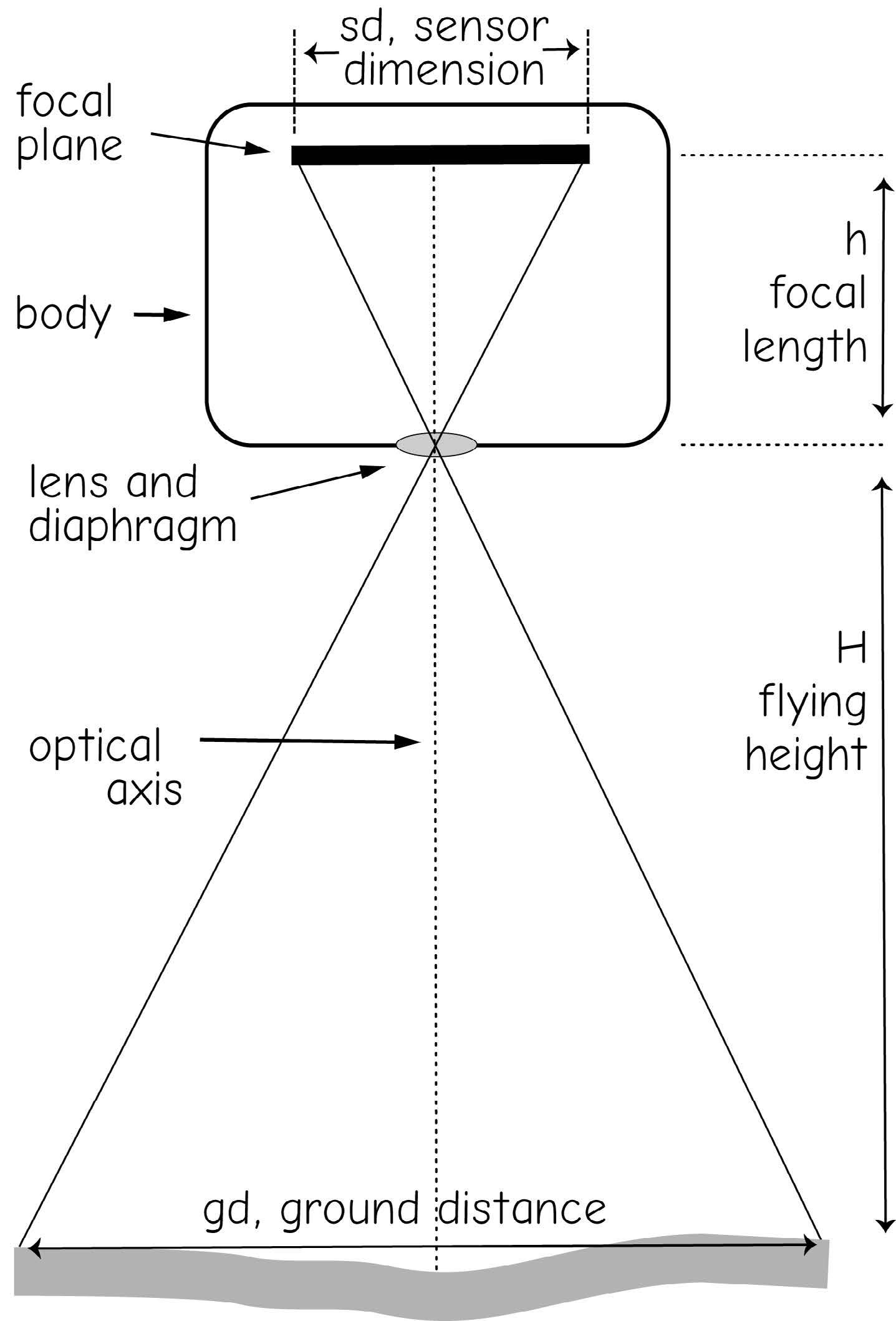
Figure 12: A simple camera (source: Bolstad, 2016)

Image extent is the area covered by an image, and depends on the physical size of the sensing area or element (sd in Figure 17), the camera focal length ($h$), and the flying height ($H$), according to:

$gd=sd*H/h$. (9.1)

The extent depends on the physical size of the recording media, sd, (e.g., 5 x 5 cm digital sensor), and the lens system and flying height. For example, a 5 cm sensing element with a 4 cm focal length lens flown at 3000 m height (about 10,000 ft) results in an extent of approximately 3.75 by 3.75 km$^2$, or 5.1 mi$^2$ on the surface of the Earth.

Image resolution is another important concept. The resolution is the smallest object that can reliably be detected on the image. Resolution in digital cameras is often set by the pixel size, the size of individual sensing elements in an array. For example, a 5 x 5 cm array with 7000 cells in each direction will have a cell size of 0.05/7000, which is 7.1 x 10-6 m, or 7.13 $\mu$m. The realized or ground resolution on aerial images may be approximately calculated from equation (7.1), substituting cell dimension for sensor dimension, sd. In our example, if the camera has a 10 cm (0.1m) focal length, and is flown at 3000 m, the ground resolution is:

$0.21 m = 7.1 x 10-6 * 3000 / 0.1$ (9.2)

Resolution in aerial photographs is more complicated, and depends on film grain size and exposure properties, and is often tested via photographs of alternating patterns of black and white lines. At some threshold of line width, the difference between black and white lines cannot be distinguished, giving the effective resolution.

9.2.4.2 Digital Aerial Cameras

Digital aerial cameras are the most common systems used for aerial mapping, and routinely provide high-quality images (Figure 13). Film cameras were most common for the 1920s through the mid-1990s, but we are nearing the end of a transition from film to digital cameras. Digital aerial cameras provide many advantages over film cameras, including greater flexibility, easier planning and execution, greater stability, and direct to digital output. While many film cameras are still in use today, camera production has effectively ceased, and film will soon follow.

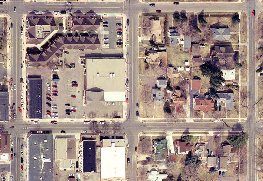
Figure 13: Digital images may provide image quality equal to or better than film images. This figure shows images collected at 15 cm resolution. Extreme detail is visible, including roof vents, curb locations, and street poles (courtesy USGS)(source: Bolstad, 2016)

Digital cameras typically consist of an electronic housing that sits atop a lens assembly (Figure 14). The lens focuses light onto charge-coupled devices (CCDs) or similar electronic scanning elements. A CCD is a rectangular array of pixels, or picture elements, that respond to light.

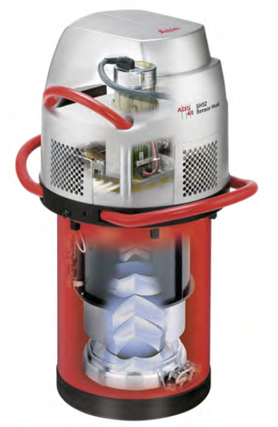
Figure 14: Digital aerial cameras are superficially similar to film aerial cameras, but typically contain many and more sophisticated electronic components - courtesy Leica Geosystems)(source: Bolstad, 2016)

The CCD is composed of layers of semiconducting material with appropriate reflective and absorptive coatings, insulators, and conducting electrodes (Figure 15). Incoming radiation passes through the coatings and into the semiconductors, dislodging electrons and creating a voltage or current. Response may be calibrated and converted to measures of light intensity. Response varies across wavelength, but can be tuned to wavelength regions by manipulating semiconductor composition. Since the pixels are in an array, the array then defines an image.

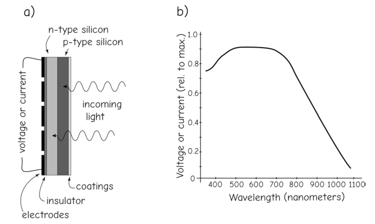
Figure 15: CCD response for a typical silicon-based receptor. The CCD is a sandwich of semiconducting layers (a, on left) that generates a current or voltage in proportion to the light received. Response varies over a wavelength region (b, on right)(source: Bolstad, 2016)

Digital cameras sometimes use a multilens cluster rather than a single lens, or they may split the beam of incoming light via a prism, diffraction grating, or some other mechanism (Figure 16). Since CCDs are typically configured to be sensitive to only a narrow band of light, multiple CCDs may be used, each with a dedicated lens and a specific waveband. Multiple CCDs typically allow more light for each pixel and waveband, but this increases the complexity of the camera system. If a multi-lens system is used, the individual bands from the multiple lenses and CCDs must be carefully coregistered, or aligned, to form a complete multiband image.

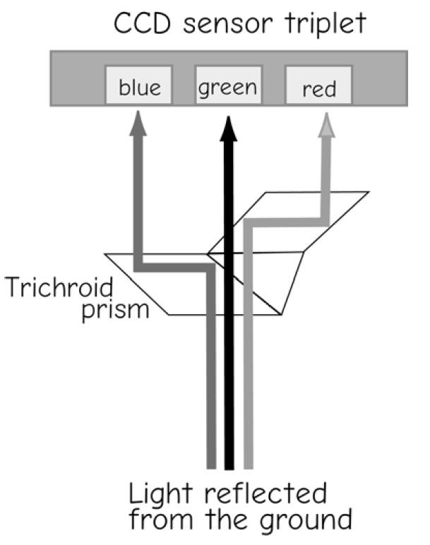
Figure 16: Digital cameras often use a prism or other mechanism to separate and direct light to appropriate CCD sensors (adapted from Leica Geosystems)(source: Bolstad, 2016)

Digital cameras most commonly collect images in the blue (0.4–0.5 $\mu$m), green (0.5–0.6 $\mu$m), or red (0.6–0.7 $\mu$m) portion of the electromagnetic spectrum. This provides an image approximately equal to what the human eye perceives. Systems may also record near-infrared reflectance (0.7–1.1 $\mu$m), particularly for vegetation mapping. The camera may also have a set of filters that may be placed in front of the lens, for example, for protection or to reduce haze.

Digital cameras typically have a computer control system, used to specify the location, timing, and exposure; record GPS and aircraft altitude and orientation information; provide data transfer and storage; and allow the operator to monitor progress and image quality during data collection (Figure 17).

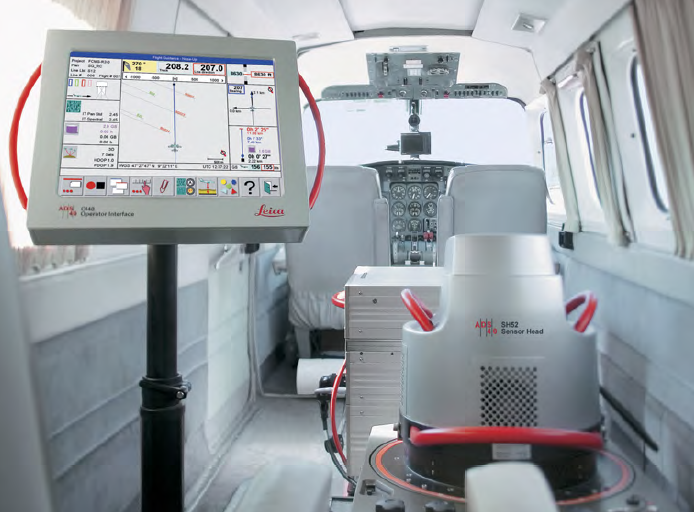
Figure 17: An example of the sophisticated system (upper left) for controlling digital image collection, here with a Leica Geosystems ADS40 digital aerial camera (lower right). These systems record and display flight paths and camera stations in real time, and may be used to plan, execute, and monitor image data collection (courtesy Leica Geosystems)(source: Bolstad, 2016)

Digital cameras may have several features to improve data quality. For example, digital cameras may employ electronic image motion compensation, combining information collected across several rows of CCD pixels. This may lead to sharper images (Figure 6-8), while reducing the likelihood of camera malfunction due to fewer moving parts. In addition, digital data may be recorded in long, continuous strips, easing the production of image mosaics.

9.2.4.3 Film and film Cameras

While most future aerial images will be collected with digital cameras, there is a vast archive of past aerial images collected with aerial film cameras.These images come in various formats, or sizes, usually specified by the edge dimension of the imaged area. Film cameras typically specify their dimensions in physical units, for example, a 240 mm (9-in) format specifies a square photograph 240 mm on a side. Cameras capable of using 240 mm film are considered large format, while smaller sizes, for example, 70 mm, were once common. Large-format cameras are most often used to take photographs for spatial data development.

Film consists of a sandwich of light-sensitive coatings spread on a thin plastic sheet. Film may be black and white, with a single layer of light-sensitive material, or color, with several layers of light-sensitive material. Each film layer is sensitive to a different set of wavelengths. These layers, referred to as the emulsions, undergo chemical reactions when exposed to light. More light energy falling on the film results in a more complete chemical reaction, and hence a greater film exposure.

Films may be categorized by the wavelengths of light they respond to. Black and white films are sensitive to light in the visible portion of the spectrum, from 0.4 to 0.7 $\mu$m, and are often referred to as panchromatic films. Panchromatic films were widely used for aerial photography because they were inexpensive and could obtain a useful image over a wide range of light conditions. True color film is also sensitive to light across the visible spectrum, but in three separate colors.

Infrared films have been developed and were widely used when differences in vegetation type were of interest. These films are sensitive through the visible spectrum and longer infrared wavelengths, up to approximately 0.95 $\mu$m.

9.2.4.4 Geometric Quality of Aerial Images

Aerial images are a rich source of spatial information for use in GIS, but most aerial images contain geometric distortion (Figure 19). Most geometrically precise maps are orthographic. An orthographic map plots the position of objects after they have been projected onto a common plane, often called a datum plane (Figure 18). Objects above or below the plane are vertically projected down or up onto the horizontal plane. Thus, the top and bottom of a building should be projected onto the same location in the datum plane. The tops of all buildings are visible, and all building sides are not. Except for overhangs, bridges, or similar structures, the ground surface is visible everywhere.

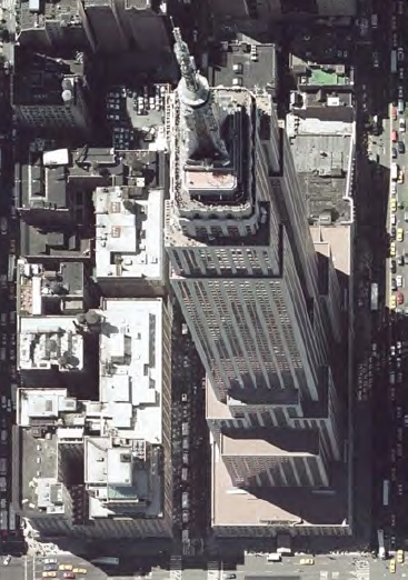
Figure 18: Tilt distortion is common on aerial and some satellite images, the result of perspective distortion when imaging the top and bottom of buildings, or any objects at different elevations.)(source: Bolstad, 2016)

Unfortunately, most aerial images provide a non-orthographic perspective view (Figure 19, left). Perspective views give a geometrically distorted image of the Earth’s surface. Distortion affects the relative positions of objects, and uncorrected data derived from aerial images may not directly overlay data in an accurate orthographic map.The amount of distortion in aerial images may be reduced by selecting the appropriate camera, lens, flying height, and type of aircraft. Distortion may also be controlled by collecting images under proper weather conditions during periods of low wind and by employing skilled pilots and operators. However, some aspects of the distortion may not be controlled, and no camera system is perfect, so there is some geometric distortion in every uncorrected aerial image. The real question becomes, “is the distortion and geometric error below acceptable limits, given the intended use of the spatial data?” This question is not unique to aerial images; it applies equally well to satellite images, spatial data derived from GPS and traditional ground surveys, or any other data.

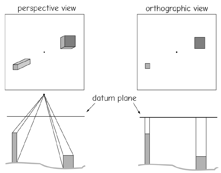
Figure 19: Orthographic (left) and perspective (right) views. Orthographic views project at right angles to the datum plane, as if viewing from an infinite height. Perspective views project from the surface onto a datum plane from a fixed viewing location.(source: Bolstad,2016)

Distortion in aerial images comes primarily from six sources: terrain, camera tilt, film deformation, the camera lens, sensor defects or other camera errors, and atmospheric bending. The first two sources of error, terrain variation and camera tilt, are usually the largest sources of geometric distortion when using an aerial mapping camera. The last four are relatively minor when a mapping camera is used, but they may still be unacceptable, particularly when the highest-quality data are required. Established methods may be used to reduce the typically dominant tilt and terrain errors and the usually small geometric errors due to lens, camera, and atmospheric distortion.

Camera and lens distortions may be quite large when nonmapping, small-format cameras are used, such as 35 mm or 70 mm format cameras. Small-format cameras can be used for GIS data input, but spatial errors are usually quite large, and great care must be taken in ensuring that geometric distortion is reduced to acceptable levels when using small-format cameras.

9.2.4.5 Terrain and Tilt Distortion in Aerial Images

Terrain variation, defined as differences in elevation within the image area, is often the largest source of geometric distortion in aerial images. Terrain variation causes relief displacement, defined as the radial displacement of objects that are at different elevations.

Figure 20 illustrates the basic principles of relief displacement. The figure shows the photographic geometry over an area with substantial differences in terrain. The reference surface (datum plane) in this example is chosen to be at the elevation of the nadir point directly below the camera, N on the ground, imaged at n on the photograph. The camera station P is the location of the camera at the time of the photograph. We are assuming a vertical photograph, meaning the optical axis of the lens points vertically below the camera and intersects the reference surface at a right angle at the nadir location.

The locations for points A and B are shown on the ground surface. The corresponding locations for these points occur at A’ and B’ on the reference datum surface. These locations are projected onto the imaging sensor or film, as they would appear in a photograph taken over this varied terrain. In a real camera the sensor is behind the lens; however, it is easier to visualize the displacement by showing the sensor in front of the lens, and the geometry is the same.

Note that the points a and b are displaced from their reference surface locations, a’ and b’. The point a is displaced radially outward relative to a’, because the elevation at A is higher than the reference surface. The displacement of b is inward relative to b’, because B is lower than the reference datum. Note that any points that have elevations exactly equal to the elevation of the reference datum will not be displaced, because the reference and ground surfaces coincide at those points.

Figure 21 illustrates the following key characteristics of terrain distortion in vertical aerial images:

Terrain distortions are radial – higher elevations are displaced outward, and lower elevations displaced inward relative to the center point.
Relief distortions affect angles and distances on an image – relief distortion changes the distances between points, and will change most angles. Straight lines on the ground will not appear to be straight on the image, and areas will expand or shrink.
Scale is not constant on aerial images – scale changes across the photograph and depends on the magnitude of the relief displacement. We may describe an average scale for a vertical aerial photograph over varied terrain, but the true scale between any two points will often differ.
A vertical aerial image taken over varied terrain is not orthographic – we cannot expect geographic data from terrain-distorted images to match orthographic data in a GIS. If the distortions are small relative to digitizing error or other sources of geometric error, then data may appear to match data from orthographic sources. If the relief displacement is large, it will add significant errors.

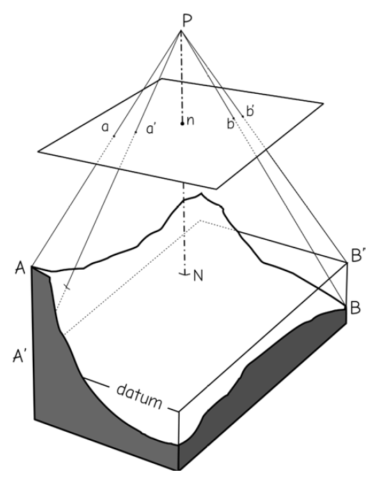
Figure 20: Geometric distortion on an aerial photograph due to relief displacement. P is the camera station, N is the nadir point. The locations of features are shifted, depending on their differences in elevation from the datum, and their distance from the nadir point. Unless corrected, this will result in non-orthometric images, and errors in location, distance, shape, and area for any spatial data derived from these images - adapted from Lillesand, Kiefer, and Chipman, 2007.)(source: Bolstad, 2016)

Camera tilt may be another large source of positional error in aerial images. Camera tilt, in which the optical axis points at a nonvertical angle, results in complex perspective convergence in aerial images. Objects farther away appear to be closer together than equivalently spaced objects that are nearer the observer (Figure 26). Tilt distortion is zero in vertical photographs, and increases as tilt increases.

Contracts for aerial mapping missions typically specify tilt angles of less than 3 degrees from vertical. Perspective distortion caused by tilt is somewhat difficult to remove, and removal tends to reduce resolution near the edges of the image. Therefore, efforts are made to minimize tilt distortion by maintaining a vertical optical axis when images are collected. Camera mounting systems are devised so the optical axis of the lens points directly below, and pilots attempt to keep the aircraft on a smooth and level flight path as much as possible. Planes have stabilizing mechanisms, and cameras may be equipped with compensating mechanics to maintain an untilted axis. Despite these precautions, tilt happens, due to flights during windy conditions, pilot or instrument error, or system design.

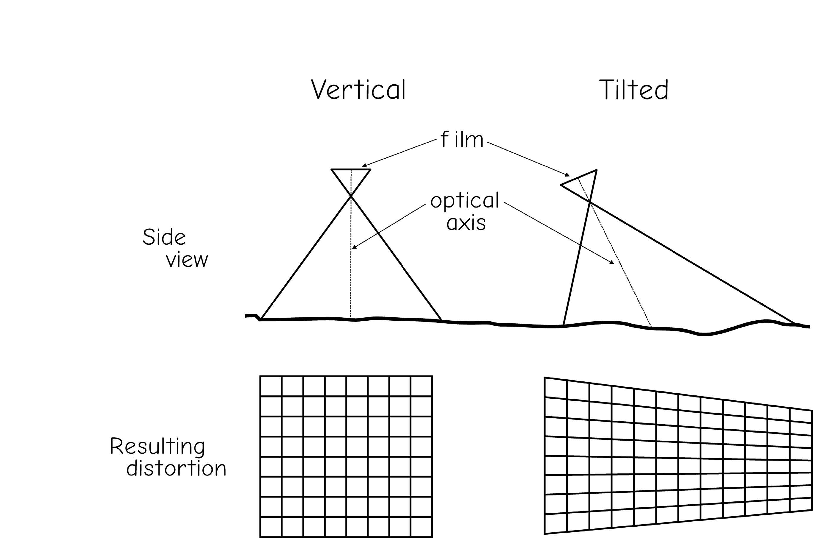
Figure 21: Image distortion caused by a tilt in the camera optical axis relative to the ground surface. The perspective distortion, shown at the bottom right, results from changes in the viewing distance across the photograph.)(source: Bolstad, 2016)

Tilt is often characterized by three angles of rotation, often referred to as omega ($\omega$), phi ($\phi$), and kappa ($\kappa$). These are angles about the $X, Y$, and $Z$ axes that define three-dimensional space (Figure 22). Rotation about the $Z$ axis alone does not result in tilt distortion, because it occurs around the axis perpendicular with the surface. If $\omega$ and $\phi$ are zero, then there is no tilt distortion. However, tilt is almost always present, even in small values, so all three rotation angles are required to describe and correct it.

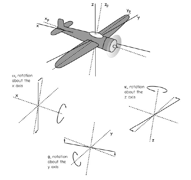
Figure 22: Image tilt angles are often specified by rotations about the $X$ axis (angle $\omega$), the $Y$ axis (angle $\phi$), and the Z axis (angle $\kappa$).)(source: Bolstad, 2016)

Tilt and terrain distortion may both occur on aerial images taken over varied terrain. Tilt distortion may occur even on vertical aerial images, because tilts up to 3 degrees are usually allowed. The overall level of distortion depends on the amount of tilt and the variation in terrain, and also on the photographic scale. Not surprisingly, errors increase as tilt or terrain increase, and as photographic scale becomes smaller.

Figure 23 illustrates the changes in total distortion with changes in tilt, terrain, and image scale. This figure shows the error that would be expected in data digitized from vertical aerial images when only applying an affine transformation, a standard procedure used to register orthographic maps. The process used to produce these error plots mimics the process of directly digitizing from uncorrected aerial images. Note first that there is zero error across all scales when the ground is flat (terrain range is zero) and there is no tilt (bottom line, left panel in Figure 28). Errors increase as image scale decreases, shown by increasing errors as you move from left to right in both panels. Error also increases as tilt or terrain increase.

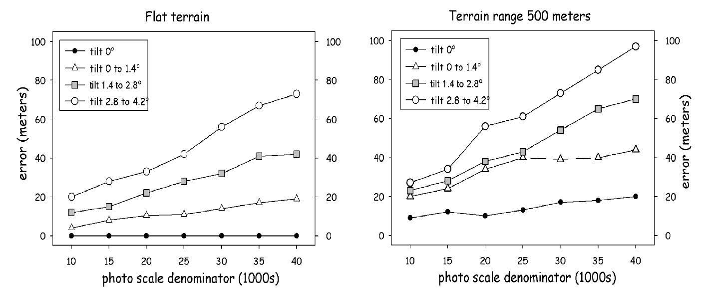
Figure 23: Terrain and tilt effects on mean positional error when digitizing from uncorrected aerial images. Distortion increases when tilt and terrain increase, and as photo scale decreases (source: Bolstad, 2016)

Geometric errors can be quite large, even for vertical images over moderate terrain (Figure 23, right side). These graphs clearly indicate that geometric errors will occur when digitizing from vertical aerial images, even if the digitizing system is perfect and introduces no error. Thus the magnitude of tilt and terrain errors should be assessed relative to the geometric accuracy required before digitizing from uncorrected aerial images.

9.2.4.6 System Errors: Media, Lens, and Camera Distortion

The film, camera, and lens system may be a significant source of geometric error in aerial images. The perfect lens–camera–detector system would exactly project the viewing geometry of the target onto the image recording surface, either film or CCD. The relative locations of features on the image in a perfect camera system would be exactly the same as the relative locations on a viewing plane an arbitrary distance in front of the lens. Real camera systems are not perfect and may distort the image. For example, the light from a point may be bent slightly when traveling through the lens, or the film may shrink or swell, both causing a distorted image.

Radial lens displacement is one form of distortion commonly caused by the camera system. Whenever a lens is manufactured there are always some imperfections in the curved shapes of the lens surfaces. These cause a radial displacement, either inward or outward, from the true image location. Radial lens displacement is typically quite small in mapping camera systems, but it may be quite large in other systems. A radial displacement curve is often developed for a mapping camera lens, and this curve may be used to correct radial displacement errors when the highest mapping accuracy is required.

Mapping camera systems are engineered to minimize systematic errors. Lenses are designed and precisely manufactured so that image distortion in minimized. Lens mountings, the detectors, and the camera body are optimized to ensure a faithful rendition of image geometry. Films are designed so that there is limited distortion under tension on the camera spools. This optimization leads to extremely high geometric fidelity in the camera/lens system. Thus, camera and lens distortions in mapping cameras are typically much smaller than other errors, for example, tilt and terrain errors, or errors in converting the image data to forms useful in a GIS. Camera-caused geometric errors may be quite high when a nonmapping camera is used, such as when photographs are taken with small-format 35 mm or 70 mm camera system. Lens radial distortion may be extreme, and these systems are likely to have large geometric errors when compared to mapping cameras. That is not to say that mapping cameras must always be used. In some circumstances the distortions inherent in small-format camera systems may be acceptable, or may be reduced relative to other errors, for example, when very large scale photographs are taken, and when qualitative or attribute information are required. However, the geometric quality of any nonmapping camera system should be evaluated prior to use in a mapping project.

9.2.4.7 Stereo Photographic Coverage

As noted above, relief displacement in vertical aerial images adds a radial displacement that depends on terrain heights. The larger the terrain differences, the larger the relief displacement. This relief displacement may be a problem if we wish to produce a map from a single photograph. Photogrammetric methods can be used to remove the distortion. However, if two overlapping photographs are taken, called a stereopair, then these photographs may be used together to determine the relative elevation differences. Relief displacement in a stereopair may be used to determine elevation and remove distortion. Many mapping projects collect stereo photographic coverage in which sequential photographs in a flight line overlap, called endlap, and adjacent flightlines overlap, called sidelap (Figure 24). Stereo photographs typically have near 60-65% endlap and 25-30% sidelap. Some digital cameras collect data in continuous strips and so only collect sidelap.

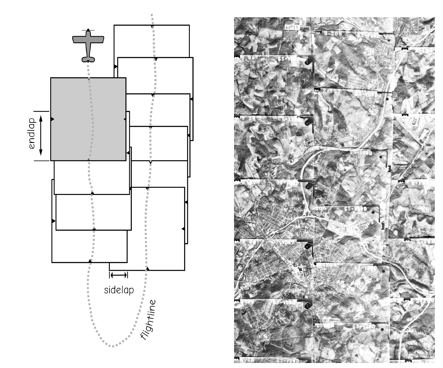
Figure 24: Aerial images often overlap to allow three-dimensional measurements and the correction of relief displacement. Sidelap and endlap are demonstrated in the figure (left) and the photomosaic (right).(source: Bolstad, 2016)

A stereomodel is a three-dimensional perception of terrain or other objects that we see when viewing a stereopair. As each eye looks at a different, adjacent photograph from the overlapping stereopair, we observe a set of parallax differences, and our brain may convert these to a perception of depth. When we have vertical aerial images, the distance from the camera to each point on the ground is determined primarily by the elevations at each point on the ground. We may observe parallax for each point and use this parallax to infer the relative elevation for every point.

Stereo viewing creates a three-dimensional stereomodel of terrain heights, with our left eye looking at the left photo and our right eye looking at the right photo. The three-dimensional stereomodel can be projected onto a flat surface and the image used to digitized a map. We may also interpret the relative terrain heights on this three-dimensional surface, and thereby estimate elevation wherever we have stereo coverage. We can use stereopairs to draw contour lines or mark spot heights. This has historically been the most common method for determining elevation over areas larger than a few hundred hectares.

Stereomodels are visible in stereopairs due to parallax, a shift in relief displacement due to a shift in observer location. illustrates parallax (Figure 25). The block (closer to the viewing locations) appears to shift more than the sphere when the viewing location is changed from the left to the right side of the objects. The displacement of any given point is different on the left vs. the right ground views because the relative viewing geometry is different. Points are shifted by different amounts, and the magnitude of the shift depends on the distance from the observer (or camera) to the objects. This shift in position with a shift in viewing location is by definition the parallax, and is the basis of depth perception.

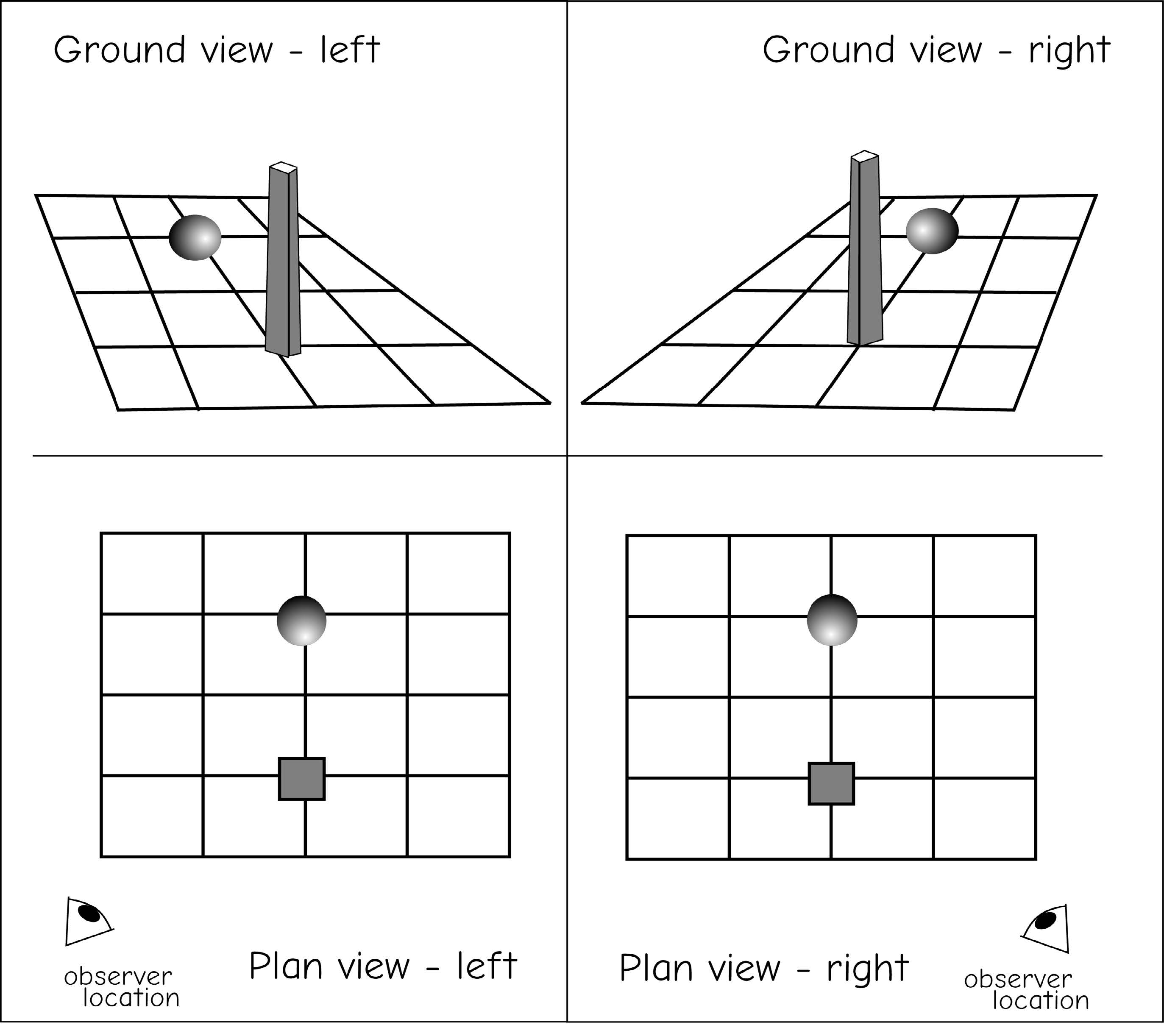
Figure 25: An illustration of parallax, the apparent relative shift in the position of objects with a shift in the viewer’s position. Objects that are farther away (sphere, above), appear to shift more when a viewer changes position. This is the bases of stereo depth perception. (source: Bolstad, 2016)

9.2.4.8 Geometric Correction of Aerial Images

Due to the geometric distortions described above, it should be quite clear that uncorrected aerial images should not be used directly as a basis for spatial data collection under most circumstances. Points, lines, and area boundaries may not occur in their correct relative positions, so length and area measurements may be incorrect. These distortions are a complex mix of terrain and tilt effects, and will change the locations, angles, and shapes of features in the image and any derived data. Worse, when spatial data derived from uncorrected photographs are combined with other sources of geographic information, features may not occur at their correct locations. A river may fall on the wrong side of a road or a city may be located in a lake. Given all the positive characteristics of aerial images, how do we best use this rich source of information? Fortunately, photogrammetry provides the tools needed to remove geometric distortions from photographs. Figure 26 illustrates the distortion in an image of a straight pipeline right-of-way, bent on the image by differences in height from valleys to rigdetops (left). Knowledge of image geometry allows us to correct the distortion (Figure 26 right).

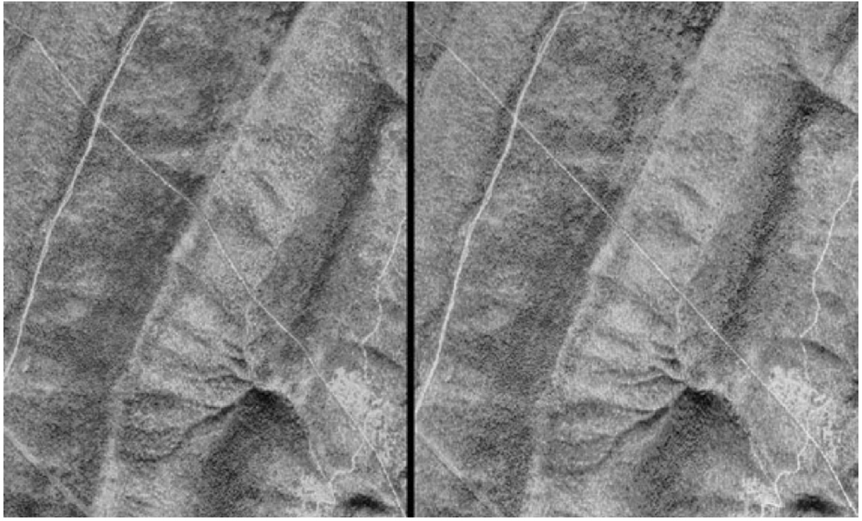
Figure 26: An example of distortion removal when creating an orthoimage. A nearly straight pipeline right-of-way spans uncorrected (left) and corrected (right) images, from the lower right to upper left in each image. The path appears bent in the image on the left as it alternately climbs ridges and descends into valleys. Using equations described in this section, these distortions may be removed, resulting in the orthographic image on the right, showing the nearly straight pipeline trajectory (courtesy USGS). (source: Bolstad, 2016)

These corrections depend on two primary sets of measurements. First, the location of each image’s perspective center or focal center must be known. This is approximately the location of the camera focal point at the time of imaging. It can be determined from precise GNSS, or deduced from ground measurements. Second, some direct or indirect measurement of terrain heights must be collected. These heights may be collected at a few points, and stereopairs used to estimate all other heights, or they may be determined from another source, for example, a previous survey, radar, or LiDAR systems described later in this chapter. Armed with perspective center and height measurements, we may correct our aerial images.

Geometric correction of aerial images involves calculating the distortion at each point, and shifting the image location to the correct orthographic position. Consider the tower in Figure 27. The bottom of the tower at $B$ is imaged on the photograph at point $b$, and the top of the tower at point $A$ is imaged on the photograph at point a. Point $A$ will occur on top of point $B$ on an orthographic map. If we consider the flat plane at the base of the tower as the datum, we can use simple geometry to calculate the displacement from a to b on the image. We’ll call this displacement d, and go through an explanation of the geometry used to calculate the displacement.

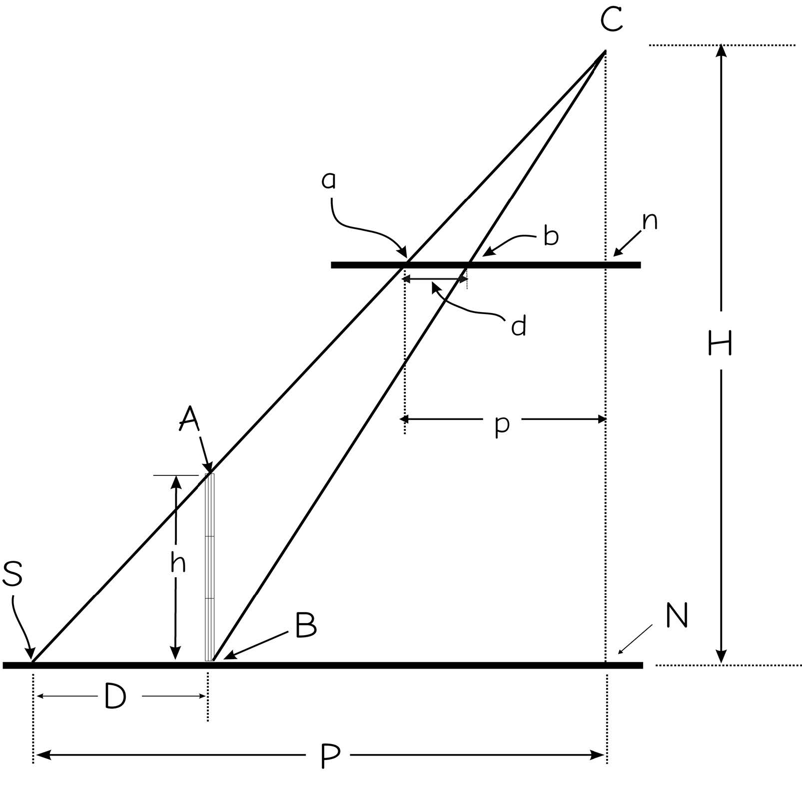
Figure 27: Relief displacement may be calculated based on geometric measurement. Similar triangles $S-N-C$ and $a-n-C$ relate heights and distances in the photograph and on the ground. We usually know flying height, H, and can measure d and p on the photograph. (source: Bolstad, 2016)

Observe the two similar triangles in Figure 32, one defined by the points $S-N-C$, and one defined by the points $a-n-C$. These triangles are similar because the angles are equal, that is, the interior angle at $n$ and $N$ are both 90$^o$, the triangles share the angle at $C$, and the interior angle at S equals the interior angle at $a$. $C$ is the focal center of the camera lens, and may be considered the location through which all light passes. The film in a camera is placed behind the focal center; however, as in previous figures, the film is shown here in front of the focal center for clarity. Note that the following ratios hold for the similar triangles:

$D/P=h/H$ (9.3)

and also

$d/p=D/P$ (9.4)

$d/p=h/H$ (9.5)

rearranging

$d=p*h/H$ (9.6)

where: $d$ = displacement distance $p$ = distance from the nadir point, $n$, on the vertical photo to the imaged point $a$ $H$ = flying height $h$ = height of the imaged point

We usually know the flying height, and can measure the distance $p$. If we can get $h$, the height of the imaged point above the datum, then we can calculate the displacement. We might climb or survey the tower to measure its height, $h$, and then calculate the photo displacement by equation (9.6). Relief displacement for any elevated location may be calculated provided we know the height. Heights have long been calculated by measurements from stereopairs, but are increasingly measured using LiDAR, described later in this chapter. These heights and equations are used to adjust the positional distortion due to elevation, “moving” imaged points to an orthographic position.

Equation 9.4 applies to vertical aerial images. When photographs are tilted, the distortion geometry is much more complicated, as are the equations used to calculate tilt and elevation displacement. Equations may be derived that describe the threedimensional projection from the terrain surface to the two-dimensional film plane. These equations and the methods for applying them are part of the science of photogrammetry, and will not be discussed here.

Digital orthophotographs are most often produced using a softcopy photogrammetric workstation (Figure 28). This method uses digital (softcopy) images, either scanned versions of aerial images or images from a digital aerial camera. Softcopy photogrammetry uses mathematical models of photogeometry to remove tilt, terrain, camera, atmospheric, and other distortions from digital images. Control points are identified on sets of photographs, stereomodels developed, and geometric distortions estimated. These distortions are then removed, creating an orthophotograph.

The correction process requires the measurement of the image coordinates and their combination with ground $x, y$, and $z$ coordinates. Image coordinates may be measured using a physical ruler or calipers; however, they are most often measured using digital methods. Typically images are taken with a digital camera, or if taken with a film camera, the images are scanned. Measurements of image $x$ and $y$ are then determined relative to some image-specific coordinate system. These measurements are obtained from one or many images. Ground $x, y$, and $z$ coordinates come from precise ground surveys.

A set of equations is written that relates image $x$ and $y$ coordinates to ground $x, y$, and $z$ coordinates. The set of equations is solved, and the displacement calculated for each point on the image. The displacement may then be removed and an orthographic image or map produced. Distances, angles, and areas can be measured from the image. These orthographic images, also known as orthophotographs or digital orthographic images, have the positive attributes of photographs, with their rich detail and timely coverage, and some of the positive attributes of cartometric maps, such as uniform scale and true geometry.

Multiple images or image strips may be analyzed, corrected, and stitched together into a single mosaic. This process of developing photomodels of multiple images at once utilizes interrelated sets of equations to find a globally optimum set of corrections across all images.

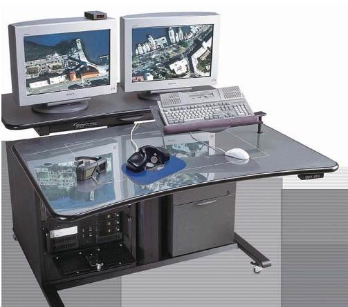
Figure 28: Digital Photogrammetric Workstation (source: http://www.dammaps.com/Images/KLT-Softcopy.jpg)

9.2.4.9 Photo Interpretation

Aerial images are useful primarily because we may use them to identify the position and properties of interesting features. Once we have determined that the film and camera system meet our spatial accuracy and information requirements, we need to collect the photographs and interpret them. Photo (or image) interpretation is the process of converting images into information. Photo interpretation is a well-developed discipline, with many specialized techniques. We will provide a very brief description of the process.

Interpreters use the size, shape, color, brightness, texture, and relative and absolute location of features to interpret images (Figure 29). Differences in these diagnostic characteristics allow the interpreter to distinguish among features. In the figure, the polygon near the center of the image labeled Pa-C, a pasture, is noticeably smoother than the polygons surrounding it, and the polygon above it labeled As-Y1 shows a finer-grained texture, reflecting smaller tree crowns than the polygon labeled NH-M11 above it and to the left. Different vegetation types may show distinct color or texture variations, road types may be distinguished by width or the occurrence of a median strip, and building types may be defined by size or shape.

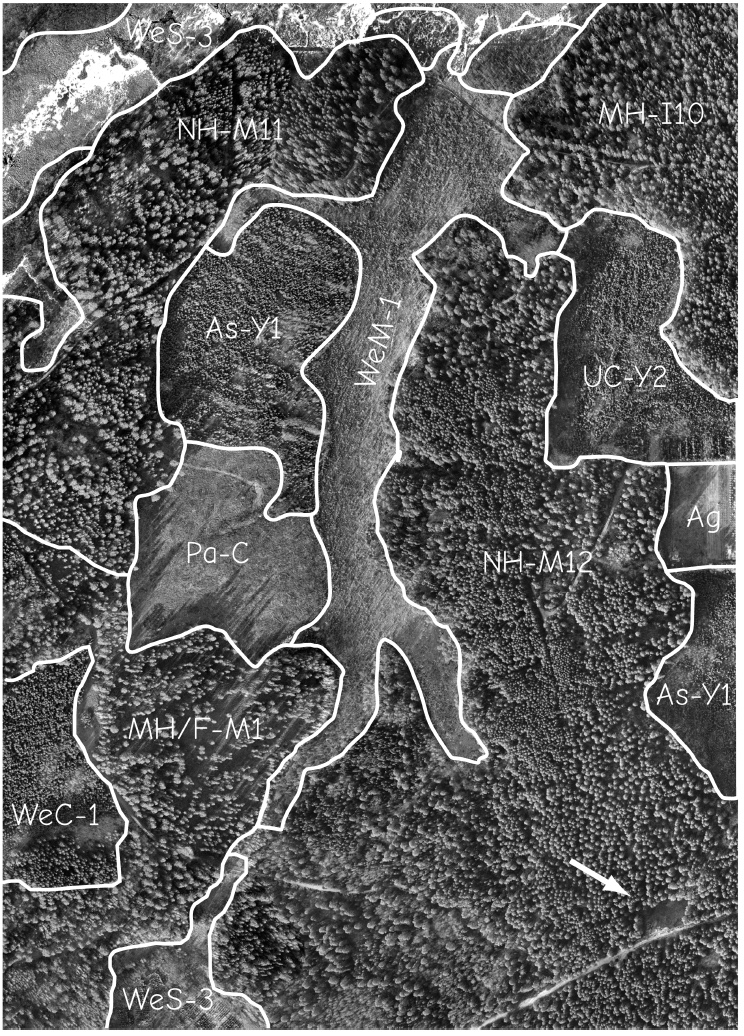
Figure 29: Photo interpretation is the process of identifying features on an image. Photo interpretation in support of GIS typically involves digitizing the points, lines, or polygons for categories of interest from a georeferenced digital or hardcopy image. In the example above, the boundaries between different vegetation types have been identified based on the tone and texture recorded in the image. The arrow at the lower right shows an “inclusion area”, not delineated because it is smaller than the minimum mapping unit. (source: Bolstad, 2016)

The proper use of all the diagnostic characteristics requires that the photo interpreter develop some familiarity with the features of interest. For example, it is difficult to distinguish the differences between many crop types until the interpreter has spent time in the field, photos in hand, comparing what appears on the photographs with what is found on the ground. This “ground truth” is invaluable in developing the local knowledge required for accurate image interpretation. When possible, ground visits should take place contemporaneously with the photographs. However, this is often not possible, and sites may only be visited months or years after the photographs were collected. The affects of changes through time on the ground-to-image comparison must then be considered.

Photo interpretation most often results in a categorical or thematic map. Identified features are assigned to one of a set of discrete classes. A crop may be corn or soybean, a neighborhood classed as urban or suburban, or a forest as evergreen or deciduous. Mixed classes may be identified, for example, mixed urban–rural, but the boundaries between features of this class and the other finite numbers of categories are discrete. Photo interpretation requires we establish a target set of categories for interpreted features. If we are mapping roads, we must decide what classes to use; for example, all roads will be categorized into one of these classes: unpaved, paved single lane, paved undivided multi lane, and paved divided multi lane. These categories must be inclusive, so that in our photos there must be no roads that are multi lane and unpaved. If there are roads that do not fit in our defined classes, we must fit them into an existing category, or we must create a category for them.

Photo interpretation also requires we establish a minimum mapping unit (MMU). A minimum mapping unit defines the lower limit on what we consider significant, and usually defines the area, length, and/or width of the smallest important feature. The arrow in the lower right corner of Figure 33 points to a forest opening smaller than our minimum mapping unit for this example map. We may not be interested in open patches smaller than 0.5 ha, or road segments shorter than 50 m long. Although they may be visible on the image, features smaller than the minimum mapping unit are not delineated and transferred into the digital data layer.

Finally, photo interpretation to create spatial data requires a method for entering the interpreted data into a digital form. Onscreen digitizing is a common method. Point, line, and area features interpreted on the image may be manually drawn in an editing mode, and captured directly to a data layer. On-screen digitizing requires a digital image, either collected initially, or by scaling a hardcopy photograph.

Another common method consists of interpretation directly from a hardcopy image. The image may be attached to a digitizing board and features directly interpreted from the image during digitizing. This entails either drawing directly on the image or placing a clear drafting sheet and drawing on the sheet. The sheet is removed on completion of interpretation, taped to a digitizing board, and data are then digitized as with a hardcopy map. Care must be taken to carefully record the location of control features on the sheet so that it may be registered.

9.3 Satellite Images

In many respects satellite images are similar to aerial images when used in a GIS. The primary motivation is to collect information regarding the location and characteristics of features. However, there are important differences between photographic and satellite-based scanning systems used for image collection, and these differences affect the characteristics and hence uses of satellite images.

Satellite scanners have several advantages relative to aerial imaging systems. Satellite scanners also have a very high perspective, which significantly reduces terrain-caused distortion. Equation 9.4 shows the terrain displacement ($d$) on an image is inversely related to the flying height ($H$). Satellites have large values for $H$, typically 600 km (360 mi) or more above the Earth’s surface, so relief displacements are correspondingly small. Because satellites are flying above the atmosphere, their pointing direction (attitude control) is very precise, and so they can be maintained in an almost perfect vertical orientation.

There may be a number of disadvantages in choosing satellite images instead of aerial images. Satellite images typically cover larger areas, so if the area of interest is small, costs may be needlessly high. Satellite images may require specialized image processing software. Acquisition of aerial images may be more flexible because a pilot can fly on short notice. Many aerial images have better effective resolution than satellite images. Finally, aerial images are often available at reduced costs from government sources. Many of these disadvantages of using satellite images diminish as more, higher-resolution, pointable scanners are placed in orbit.

9.3.1 Basic Principles of Satellite Image Scanners

Scanners operate by pointing the detectors at the area to be imaged. Each detector has an instantaneous field of view (IFOV), that corresponds to the size of the area viewed by each detector (Figure 30). Although the IFOV may not be square and a raster cell typically is square, this IFOV may be thought of as approximately equal to the raster cell size for the acquired image. The scanner builds a two-dimensional image of the surface by pointing a detector or detectors at each cell and recording the reflected energy. Data are typically collected in the across-track direction, perpendicular to the flight path of the satellite, and in the along-track direction, parallel to the direction of travel (Figure 30). Several scanner designs achieve this across- and along-track scanning. Some older designs use a spot detector and a system of mirrors and lenses to sweep the spot across track. The forward motion of the satellite positions the scanner for the next swath in the along-track direction. Other designs have a linear array of detectors – a line of detectors in the acros-strack direction. The across-track line is sampled at once, and the forward motion of the satellite positions the array for the next line in the along-track direction. Finally, a two-dimensional array may be used, consisting of a rectangular array of detectors. Reflectance is collected in a patch in both the across-track and the along-track directions.

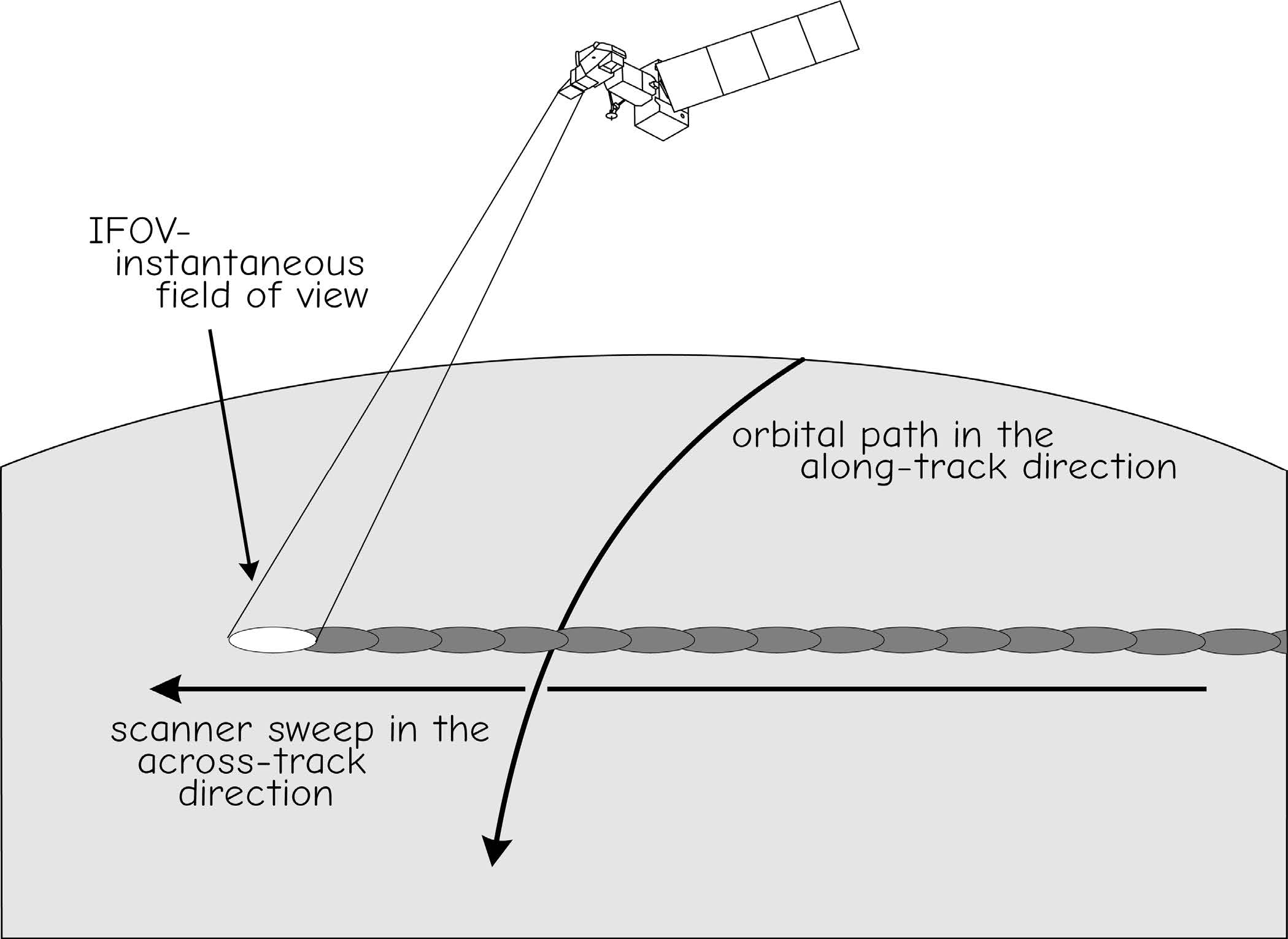
Figure 30: A spot scanning system. The scanner sweeps an instantaneous field of view (IFOV) in an across-track direction to record a multispectral response. Subsequent sweeps in an along-track direction are captured as the satellite moves forward along the orbital path. (source: Bolstad, 2016)

A remote sensing satellite also contains a number of other subsystems to support image data collection. A power supply is required, typically consisting of solar panels and batteries. Precise altitude and orbital control are needed, so satellites carry navigation and positioning subsystems. Sensors evaluate satellite position and pointing direction, and thrusters and other control components orient the satellite. There is a data storage subsystem, and a communications subsystem for transmitting data back to

Earth and for receiving control and other information. All of these activities are coordinated by an onboard computing system.

Several remote sensing satellite systems have been built, and data have been available for land surface applications since the early 1970s. The detail, frequency, and quality of satellite images have been improving steadily, and there are several satellite remote sensing systems currently in operation. Satellite data are often nominally collected in a path/row system. A set of approximately north-south paths are designated, with approximately east-west rows identified across the paths. Satellite scene location may then be specified by a path/row number (Figure 31). Satellite data may also be ordered for customized areas, depending on the flexibility of the acquisition system. Because most satellites are in near-polar orbits, images overlap most near the poles. Adjacent images typically overlap a small amount near the equator. The inclined orbits are often sun synchronous, meaning the satellite passes overhead at approximately the same local time.

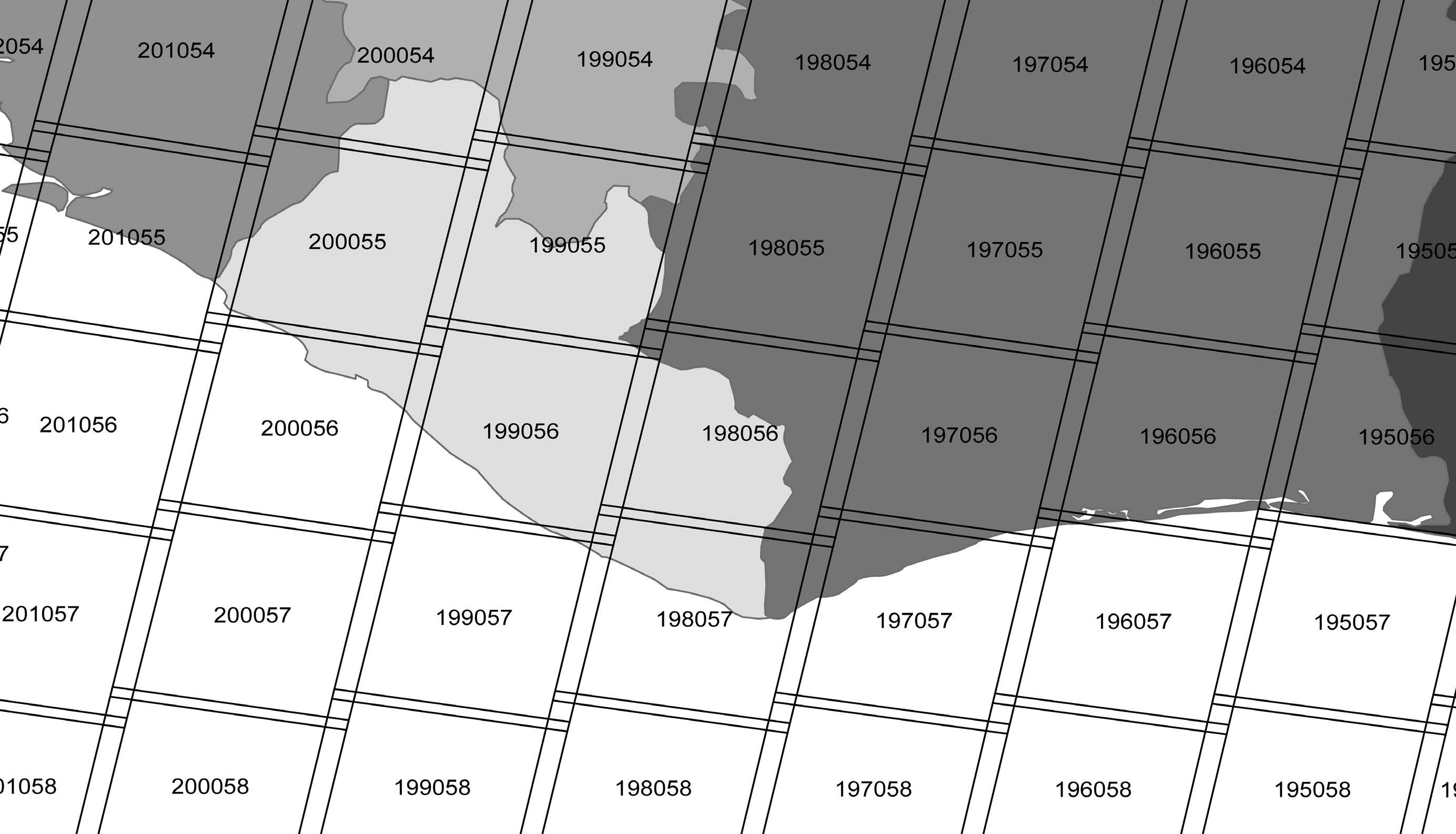
Figure 31: A portion of the path and row layout for the Landsat satellite systems. Each slightly overlapping, labelled rectangle corresponds to a satellite image footprint. (source: Bolstad, 2016)

Satellite data parameters

When selecting suitable remote sensing data for a specific application, it is necessary to focus on several basic parameters of satellite images. The first is spatial resolution (Figure 32), which defines how large an area on the earth’s surface corresponds to one pixel in an image.

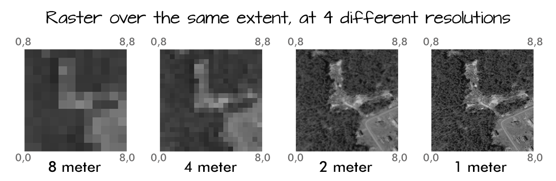
Figure 32: Spatial resolution (zdroj: National Ecological Observatory Network)

The higher the spatial resolution, the more detail can be seen in the image. In this respect, low-resolution satellites capturing images with a pixel size larger than 1 km can be distinguished. Images of this spatial resolution are not very detailed, but they capture a large part of the earth’s surface and imaging can be done very often, even several times a day. This type of resolution is typical of meteorological satellites such as NOAA or MetOp. Medium resolution satellites have a pixel size in the range of 100 to 250 meters. They are used mainly for studies of regional scope, while the scanning of one surface is repeated in the order of several days. The Envisat satellite, for example, has a medium spatial resolution. The pixel size of high-resolution data is about 10 to 50 meters, such as Landsat or SPOT satellites. Medium and high resolution images are mainly used to monitor the earth’s surface (e.g. ocean monitoring, vegetation health or regional mapping). Using very high resolution satellites, the earth’s surface can already be monitored in great detail, the pixel size in this case is 5 meters and less. Such detailed data are used mainly for spatial planning or detailed local mapping. Very high resolution satellites are mostly operated by commercial entities and acquire data to order.

Another important parameter of remote sensing data is temporal resolution (Figure 33), which indicates with which time period they are acquired for the same area. While low spatial resolution meteorological satellites can take images of the same area several times a day, in the case of satellites with a resolution of several meters, the measurements are repeated very little.

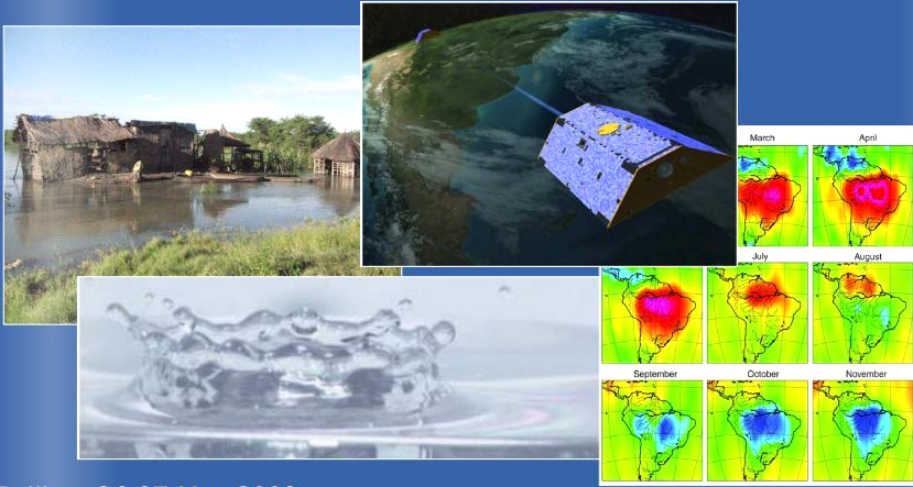
Figure 33: Temporal resolution (source: https://www.yumpu.com/en/document/read/35672411/grace-temporal-resolution-futurewater)

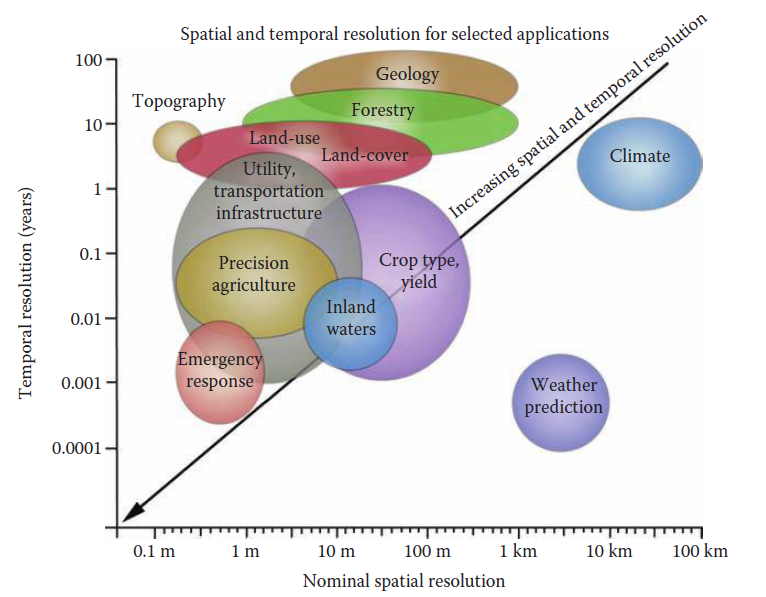
Figure 34: Spatial and Temporal Resolution for Selected Applications (source: https://www.yumpu.com/en/document/read/35672411/grace-temporal-resolution-futurewater)

Spectral resolution specifies the number of spectral bands in which the sensor can capture radiation. The number of bands is not only important aspect of spectral resolution: it is aslo essential the position of the bands in the electromagnetic spectrum. In this regard, it is possible to distinguish between multispectral data that contain several units of bands in the order of tens of nm and hyperspectral data that contain several tens to hundreds of spectral bands with a width of several nm. Hyperspectral images therefore provide very detailed information about the earth’s surface (Figure 35).

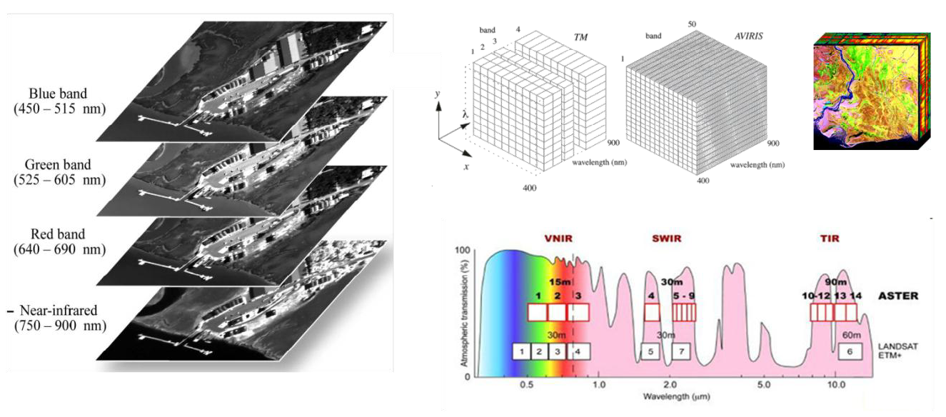
Figure 35: Spectral resolution (zdroj: González et al., 2010)

The last one is radiometric resolution which describes accuracy and minimum change possible in radiance measurement.

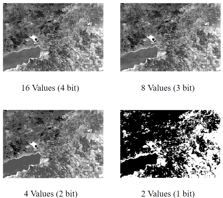
Figure 36: Radiometric resolution (source: https://commons.wikimedia.org/wiki/File:Decreasing_radiometric_resolution_from_L7_15m_panchromatic.svg)

9.3.1.1 High Resolution Satellite Systems

There is a large and growing number of high resolution satellite systems, here rather arbitrarily defined here as those with a resolution finer than 3 m. This is the resolution long available on the largest-scale aerial photographs, and used for fine-scale mapping of detailed features such as sidewalks, houses, roads, individual trees, and small area landscape change. Commercial systems providing 30 cm resolution are in operation, with higher resolution systems in the offing. This detail blurs the distinction between satellite and photo-based images.

Images from high-resolution satellite systems may provide a suitable source for spatial data in a number of settings. These images provide substantial detail of manmade and natural features, and match the spatial resolution and detail of high-accuracy GNSS receivers. They are typically required by cities and businesses for fine-scale asset management, for example, in urban tree inventories, construction monitoring, or storm damage assessment. Nearly all the systems have pointable optics or satellite orientation control, resulting in short revisit times, on the order of one to a few days.

Spectral range, price, availability, reliability, flexibility, and ease of use may become more important factors in selecting between aerial images and high-resolution satellite images. Satellite data are attractive when collecting data for larger areas, or where it is unwise or unsafe to operate aircraft, or because data for large areas may be geometrically corrected for less cost and time. Aerial images may be preferred when resolutions of a few centimeter are needed, or for smaller areas, under narrower acquisition windows, or with instrument clusters not possible from space. Aerial images will not be completely replaced by satellites, but they may well pushed towards the finest resolutions and county-sized or smaller collections.

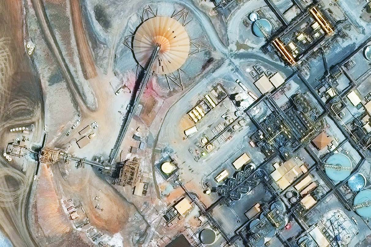
Figure 37: 0.3 m resolution image of the Kalgoolie Mine in Western Australia, demonstrating the detail available from the highest-resolution satellite imaging systems (courtesy Digital Globe. (source: Bolstad, 2016)

As of late 2015 there are several operational satellite systems capable of global image acquisition at 1 m resolution or better, including WorldView, GeoEye, Pleiades, and SPOT. These satellites and related systems are predominantly commercial enterprises, funded and operated by businesses. There are several recently decommissioned high-resolution systems for which archive data are available and still useful, including the Ikonos satellite that operated from 1999 through early 2015, and the Quickbird system, operational from 2001 through early 2015.

The Worldview-3 satellite currently provides the highest resolution available on a global basis, with a maximum resolution of 31 cm provided as panchromatic images, with addition of eight bands at a 1.24 m resolution, eight short-wave infrared bands at 3.7 m resolution for haze and smoke penetration, and 12 bands at 30 m resolution. Images are collected in a 13.1 km swath width at nadir, and due to satellite reorientation has a revisit time of less than a day, with effective global coverage on a 4-day basis. Off-nadir resolution is poorer than 30 cm, but can image the entire globe at better than 50 cm resolution in a 4.5 day period. Images are collected at approximately 10:30 a.m. local time, a common characteristic of these polar orbiting, sun-synchronous systems.

Worldview-1 and -2 preceded -3, and are still collecting data. WorldView-1 provides 0.5 m panchromatic images , while the Worldview-2 provides 0.46 m panchromatic and multispectral images at 1.8 m (Figure 6- 29). Data are collected as often as a 1.7 day return interval when providing a 1 m resolution, and 6 days with a 0.5 m resolution. Images have a swath width of approximately 17 km.

GeoEye-1 was launched in mid-2008 into a sun-synchronous orbit with a local collection time near 10:30 a.m. Image resolution has changed with time, but it currently collects panchromatic images with a 46 cm resolution and multispectral images spanning the blue through near-infrared portions of the spectrum at a 1.84 m resolution. There is a nominal 15.2 km scan width at nadir, and off-nadir imaging allows return intervals of as short as 2 days. Although the system has a 7 year design life, it may well operate much longer, given satellite imaging systems have often functioned to double their designed interval.

Pleiades-1 and -2 were launched in late 2011 and 2012 by a European consortium, with a five-year design life. The system provides 50 cm panchromatic and 2 m multispectral data in blue through near-infrared bands, with a 20 km swath width at nadir. Sun-synchronous orbital planes are offset by 180o, with a pointable satellite, allowing daily revisits by the constellation.

Another set of high-resolution images come from the Systeme Pour l’Observation de la Terre (SPOT), versions SPOT-6 and SPOT-7. These are an evolution of a set of mid resolution satellites, SPOT-1 through -5, described in the next section. The high-resolution satellites carry a 1.5 m panchromatic and 6 m resolution multispectral scanner, the latter with four bands spanning the visible through near-infrared spectrum. SPOT has a 60 km swath width at nadir. Note that this larger swath width provides 15 to 40 times the area coverage of the highest resolution satellites, and illustrates a more general trade-off between satellite image resolution and the area covered by each image. The set of SPOT satellites has a daily revisit capability, completely covering the Earth’s landmasses every two months.

A number of high-resolution satellite imaging systems have a local focus. The KOMPSAT-2 satellite is designed to collect data primarily over eastern Asia, and provides 1 m resolution panchromatic and 4 m multispectral data. The Cartosat-2 satellite, launched in 2007, provides 0.9 m resolution panchromatic data, primarily focused on south Asia. There are several new systems planned or in progress. A DMC3 satellite, by Surrey Satellite Technology Ltd., was first launched in mid-2015 and provides 1 m panchromatic and 4 m multispectral data from a 651 km, sun-synchronous orbit, in a 24 km swath width. SSTL planned a constellation of three satellites to provide more frequent coverage, with full system deployment by 2017.

Skysat-1 was launched in late 2013 and is notable for providing high-resolution images based on a small satellite, low cost approach. This approach may lead to both a larger constellation of satellites with more frequent revisits, and lower-priced images. Currently there is a planned constellation of 15 satellites, with launches scheduled at least through 2018. Skysat provides a 90 cm single-band panchromatic mode and four, 2 m resolution multispectral bands, the latter in the blue through near-infrared region. There is a nominal 8 km swath width at nadir of the multispectral data, and 2 km for panchromatic images. Repeat intervals will depend on the number of satellites deployed. Planet Labs carries this notion of a constellation of small, inexpensive, high-resolution satellites further, with a planned fleet of more than 130 “dove” satellites, approximately the size of a rural route mailbox, inexpensively deployed in clusters. First satellites were launched in 2013, with a group deployment of 28 satellites in 2014, and the full constellation expected some time by the end of 2015. The system specifies a 3 to 5 m resolution image, spanning the high to mid resolution categories. Daily revisit times by the constellation are planned, with images stitched together for complete global coverage, updating the mosaic on a daily basis.

9.3.1.2 Mid Resolution Satellite Systems

There are several mid resolution satellite systems, here defined as those providing images with resolutions from 5 m to less than 100 m. These are most often used for medium to broad-area analyses, for example, landcover mapping at county, regional, or national extents, or large-area wildfire or flooding management. Individual image collections are generally several tens to hundreds of kilometers on a side, and revisit times from a few days to a few weeks.

SPOT is one of the longest running, uninterrupted satellite imaging systems. The French Government led the development of SPOT, culminating in the launch of SPOT-1 in early 1986. There have since been four additional SPOT satellites, labeled two through five, placed in orbit. SPOT was the first satellite system designed to serve commercial interests, in a high-volume, production mode.

SPOT-5 is the only remaining mid-resolution satellite image system in the series, as SPOT-1 through -4 have been decommissioned. All SPOT satellites provide panchromatic mode and a high-resolution visible (HRV) mode. The panchromatic mode on SPOT-1 through SPOT-3 contained one image band in the visible wavelengths, and the HRV mode provided one band each in the green, red, and near-infrared portions of the spectrum. The panchromatic mode on these first satellites had a spatial resolution of 10 m, and the HRV mode has a spectral resolution of 20 m. SPOT-4 and SPOT-5 increased the panchromatic resolution to between 2.5 and 10 m, and added a 10 to 20m mid-infrared band to the HRV mode. This combination provides high resolution over large areas, and SPOT data are routinely used in a number of resource management, urban planning, and other applications.

The SPOT scanners have optics pointable to areas up to 27o to either side of the satellite path. This reduces revisit time to between one and five days, and allows the collection of satellite stereopairs suitable for elevation mapping.

SPOT images may also be used to create elevation data, due to the pointable sensors. Just as parallax may be used with aerial images to determine terrain heights, parallax may be measured from a satellite to estimate elevation. Scanners may point forward and back along the flight path, or across separate flight paths to image an area. The relative displacement on the image depends on the relative elevations on the ground. Careful measurements allow us to convert image displacement to elevations with little ground control. As noted earlier, SPOT-6 and SPOT-7 are successors, and they provide image data with resolutions between 1.5 m (panchromatic) and 6 m (mutlispectral). As of this writing, there are no plans to launch additional satellites at the coarser resolutions of SPOT-5, given the same 60 km footprint for successor satellites.

9.3.1.3 Landsat

The Landsat-8 satellite is the latest in the longest running series of intermediate resolution imaging satellites. Landsat-8 collects a 15 m resolution panchromatic band, 8 multi-spectral bands at 30 m in the visible, near-infrared, and mid-infrared portions of the spectrum, and two bands in the thermal infrared range with a 100 m resolution. The system has a 185 km swath width at nadir and a repeat interval of 16 days. Landsat-8 uses an instrument called the Operational Land Imager (OLI) to collect non-thermal bands. The specific bands used were selected to be compatible with previous Landsat missions, and to improve cloud detection and aerosol/atmospheric haze analysis. The OLI also increases the bit depth, or data width from 8 to 12 bits, giving a broader and more sensitive response, and clearer, more detailed images.

Because Landsat was the first Earth observing satellite system and it has operated nearly continuously since 1972, there is an image repository spanning five decades. The majority of these images are available free of charge to anyone with an internet connection, allowing long-term monitoring and analysis. Landsat-8 images are processed and added to this archive, typically within a few days of collection, resulting in an inexpensive source of broad-scale images. This long time series is particularly appropriate for change analysis, provided the differences between legacy and new data resolutions and formats are addressed.

Previous Landsat satellites have carried three primary imaging scanners. The Multispectral Scanner (MSS) was the first satellite-based land scanner, launched in 1972, and it has been carried on board Landsat satellites 1 through 5. The original MSS sensed in four spectral bands, at an 80 m resolution: a green, a red, and two infrared bands.

Starting in 1984, Landsat satellites also carried the Thematic Mapper (TM) or Enhanced Thematic Mapper (ETM+), an improvement over the MSS. TM data contain seven spectral bands (three visible, a near-infrared, two mid infrared, and a thermal band), and a 28.5 m grid-cell resolution for the first six bands. The ETM+ added a 15 m resolution panchromatic band covering the visible wavelengths. The satellites have had a 16 to 18 day return interval.

Due to disagreements on funding replacement satellites, Landsat-7 was operated well past its designed lifetime, and provided compromised data over the later years of operation. Data from the ETM+ became degraded in 2003 due to a scanning mirror failure, substantially reducing the utility of approximately the outside 30% of each image. Scenes from the high polar regions are little affected because there is much overlap between paths. However, approximately 30% of area in tropical regions is effectively unsampled by Landsat-7.

Landsat is used in many projects, worldwide, because of the breadth of radiometric bands, the large scan area for individual images, the long data record, and no-cost data. Landsat is the basis of many statewide and national land cover mapping projects, and it has been used to assess water quality in lake and coastal areas. Landsat is particularly appropriate for change detection, and much work has established methods for radiometric correction through time and across sensors, so that the time series of images may be used to map urban growth, vegetation change, and trajectories in water quality.

9.3.1.4 ResourceSat

The Indian Space Research Organization has launched a number of satellites designed for Earth observation, including the Cartosat series, previously described, and the IRS series, beginning with the IRS-1A in 1988. Early satellites were largely experimental and images not widely distributed, or classified, but two, Resourcesat-1 and Resourcesat-2, provide high-quality, large-area, moderate resolution data over much of the globe.

The ResourceSats have carried three scanners, LISS-IV with a 5.8m resolution, the LISS-III with a 23.5m resolution, and AWiFS with a 56 m resolution. [Swath])(https://www.nrcan.gc.ca/maps-tools-publications/satellite-imagery-air-photos/remote-sensing-tutorials/satellites-sensors/satellite-characteristics-orbits-and-swaths/9283) (image) width increases from 70 km through 141 km to 740 km for the three instruments, with a 5-day repeat cycle for the AWiFS sensor. The AWiFS is most commonly used outside of India, and provides blue, green, red, and near-infrared sensing bands, with 10-bit data. These images are often used for regional to national analyses because of their large image size and medium resolution, for example, by the U.S. National Agricultural Statistical Service for annual crop inventories in the United State.

9.3.1.5 RapidEye

RapidEye is a five-satellite constellation that provides images with an up to 5 m resolution, in five bands spanning the blue through near-infrared spectrum. Swath width is 77 km at nadir, with a 5.5 day repeat interval for nadir collections. A single-day repeat interval is possible for off-nadir viewing, but as with all tilted collections, at a reduced resolution. Satellites were launched simultaneously in 2008, with a seven year design life. Successor satellites are currently planned.

RapidEye is perhaps characteristic of a new era of high and mid resolution remote sensing systems. It was developed and deployed by a private entity, and ownership has changed during the system life. Although the most current technology and agile acquisition and delivery are supported, continuity of acquisition for the specific sensors is less certain. These systems may provide advantages for once-off or short-span applications, as with specific disaster assessments or annual crop mapping, but may provide disadvantages for long-term monitoring or change detection, for example, decadeslong land cover change.

9.3.1.6 Coarse-Resolution, Global Satellite Systems

There are currently two widely used, coarse-resolution sensors, the MODIS, and VEGETATION, and a third undergoing deployment, VIIRS.

Moderate Resolution Imaging Sensor (MODIS) is a NASA research system that collects data at a range of resolutions and wavebands, from visible through thermal infrared bands. Resolutions depend on bands and vary from 250 m to 1 km, and it has a repeat frequency of every one to two days for the entire Earth’s surface when images are sampled at the 1 km resolution. Thirty-six bands are collected when operated in the 1 km mode, ranging from 0.4 $\mu$m to 14.4 $\mu$m. Only two bands are collected at the 250 m resolution, one each in the red and infrared portions of the light spectrum. These are somewhat unique in that the resolution is finer than the 1 km resolution of AVHRR and most MODIS data, but substantially coarser than Landsat, SPOT, and moderate-resolution satellites. Large area coverage is possible at an intermediate level of detail when using [MODIS 250 m data.

VEGETATION was developed by the French national space agency, CNES. It collects data in the blue, red, near infrared, and short-wave infrared portions of the spectrum, with a nadir resolution of 1.15 km and a swath width of 2400 km, yielding daily coverage. The scanning system was designed specifically to monitor vegetation and physical environments for continental and larger areas, and it has been used to monitor crops, fires, storms, and other phenomena (Figure 38).

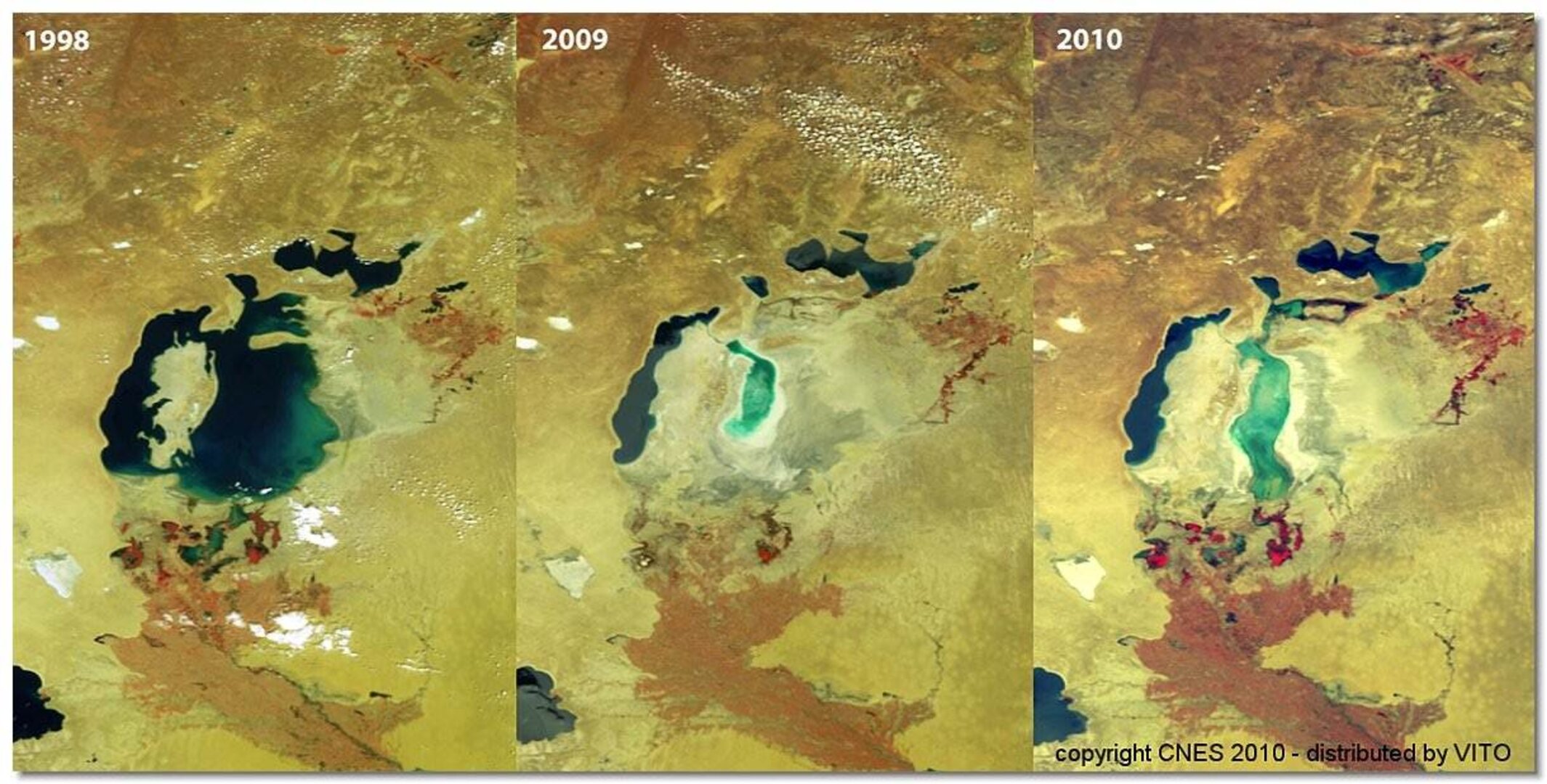
Figure 38: Aral sea monitored by Vegetation.(source: https://www.esa.int/Enabling_Support/Space_Engineering_Technology/Proba_Missions/V_for_Vegetation)

The MODIS satellites were launched in late 1999/mid 2000, with a six-year design life, so they have already outlived their mission, although they continue to function.

VIIRS is a successor instrument to MODIS, created to collect data for both weather and land surface analysis. It collects 9 visible near-infrared bands plus a day/ night band, 8 mid-infrared bands, and 4 long-wave infrared bands. VIIRS collectsdata at both 375 and 750 m resolutions, and 3040 km wide swath width, providing global coverage on a daily basis. It was developed in part as a successor to MODIS, to maintain continuity in some of the MODIS bands and products.

9.3.1.7 MERIS

MERIS is a wide-swath scanner carried aboard the ESA’s Envirosat. With 15 selectable bands at a 300m maximum resolution, a 1150 km (750 mi) swath, and 3-day global coverage, the system is in many respects an improvement on MODIS. Many of the bands are narrowly specified for a purpose, for example, several chlorophyll and sediment bands for water quality and vegetation, a yellow band, and bands to aid in atmospheric correction.

The MERIS system is designed in part for oceanographic applications, with specific bands tuned to the low-level returns from ocean targets. This leads to improved information extraction from waters, perhaps at the expense of those bands when sensing brighter land-based targets. Response saturation occurs when reflectance reaches the highest values a sensor can record.

9.3.1.8 Other Systems

There are several other airborne and satellite remote sensing systems that are operational or under development. Although some are quite specialized, each may serve as an important source of data. Some may introduce entirely new technologies, while others replace or provide incremental upgrades to existing systems. Space prevents our offering more than a brief description of these satellite systems here.

Passive optical systems - there are several remote sensing systems that are based on reflected incident radiation. These include the IRS system deployed by the Indian government, with a 5 m panchromatic band with a five-day revisit interval, three 24 m bands that span the green through near infrared portion of the spectrum, and one 70 m band in mid infrared portion of the spectrum.

A number of radar-based satellite systems have been used as a source of spatial data for GIS. Radar wavelengths are much longer than optical remote sensing systems, from approximately one to tens of centimeters, and may be used day or night, through most weather conditions. Radar images are panchromatic, because they provide information on the strength of the reflected energy at one wavelength. Radar systems have been successfully used for topographic mapping and some landcover mapping, particularly when large differences in surface texture occur, such as between water and land, or forest and recently clearcut areas. Operational systems include the ERS-1, operated by the European Space Agency; the JERS-1, by the National Space Development Agency of Japan; and the Radarsat system, developed and managed by the Canadian Space Agency.

Look at 50 Satellites in Space: Types and Uses of Satellites

9.3.2 Remote Sensing Image Processing

Digital image processing is the set of techniques applied to digital images in order to enhance visual quality or facilitate the search or extraction of information. The interest of digital image processing methods lies in two main areas of application:

the reconstruction or improvement of information that provides an image to be interpreted by a human being, and
information processing of a scene to allow automatic analysis by a machine.

Digital image processing includes the set of techniques for processing and analysing images by using computers: information extraction, sensor evaluation, statistical image evaluation, assesing/improving image quality, base data sets (e. g. for GIS) making, art making. There is a set digital image operations: geometric transformation, colour correction, image editing, image registration, image projection, compositing, image differencing, image segmentation, pattern recognition.

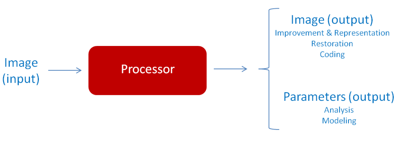
Figure 39: Image Processing System.(source: Gonzáles et al., 2013)

Let´s start with a couple of basic terms:

Sampling - is responsible for integrating in points the information which is in a given area. These points are the smallest elements that divide an image, called pixels.

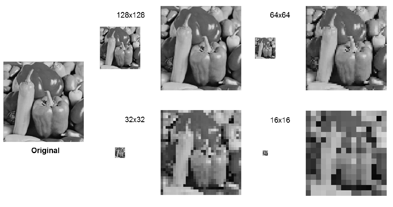
Figure 40: Image Processing Sampling. (source: Gonzáles et al., 2013)

Quantification: Once sampled the image, the value of each pixel must be digitally encoded. This process of assigning a number of levels or bits to each pixel is called “quantization” of the image.

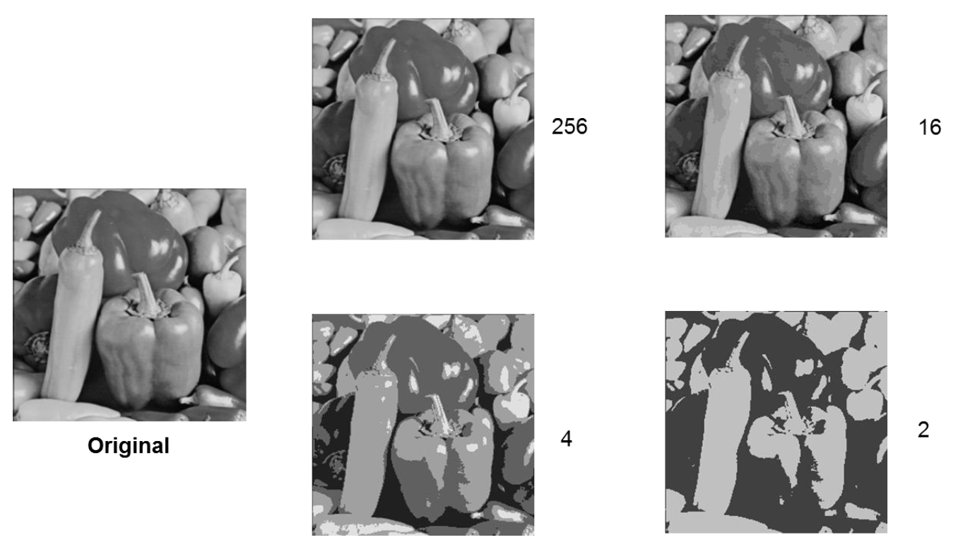
Figure 41: Image Processing Quantification. (source: Gonzáles et al., 2013)

The digital image is formed by one or more matrices (e.g., sensor bands) of numbers (DN: digital levels). That is why they are generally multidimensional functions.

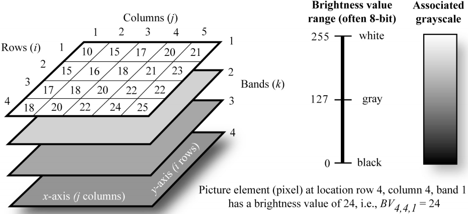
Figure 420: Digital Image. (source: https://lcluc.umd.edu/sites/default/files/lcluc_documents/ozdogan1_lcluc_8-2010_training_0.pdf)

values represented by digital images:

intensity: scalar (one band)
color: vector R,G,B (3 bands)
material properties (1 or more bands)
- X-ray images: absorption
- ultrasound images: density
- infrared images: temperature
- remote sensing images: reflectivity
Histogram - statistical distribution of the pixels of an image in terms of number of pixels for each ($DN$) possible value. It does not contain information on the spatial distribution of the pixels in the image

$hist_{ND}=\frac{count(ND)}{NxM}$.

Besides histogram we can use also univariate (mode, median, min, max, range, mean, variance, standard deviation, skewness, kurtosis) and multivariate (covariance, correlation, regression, coefficient of determination) techniques for statistical description of an image.

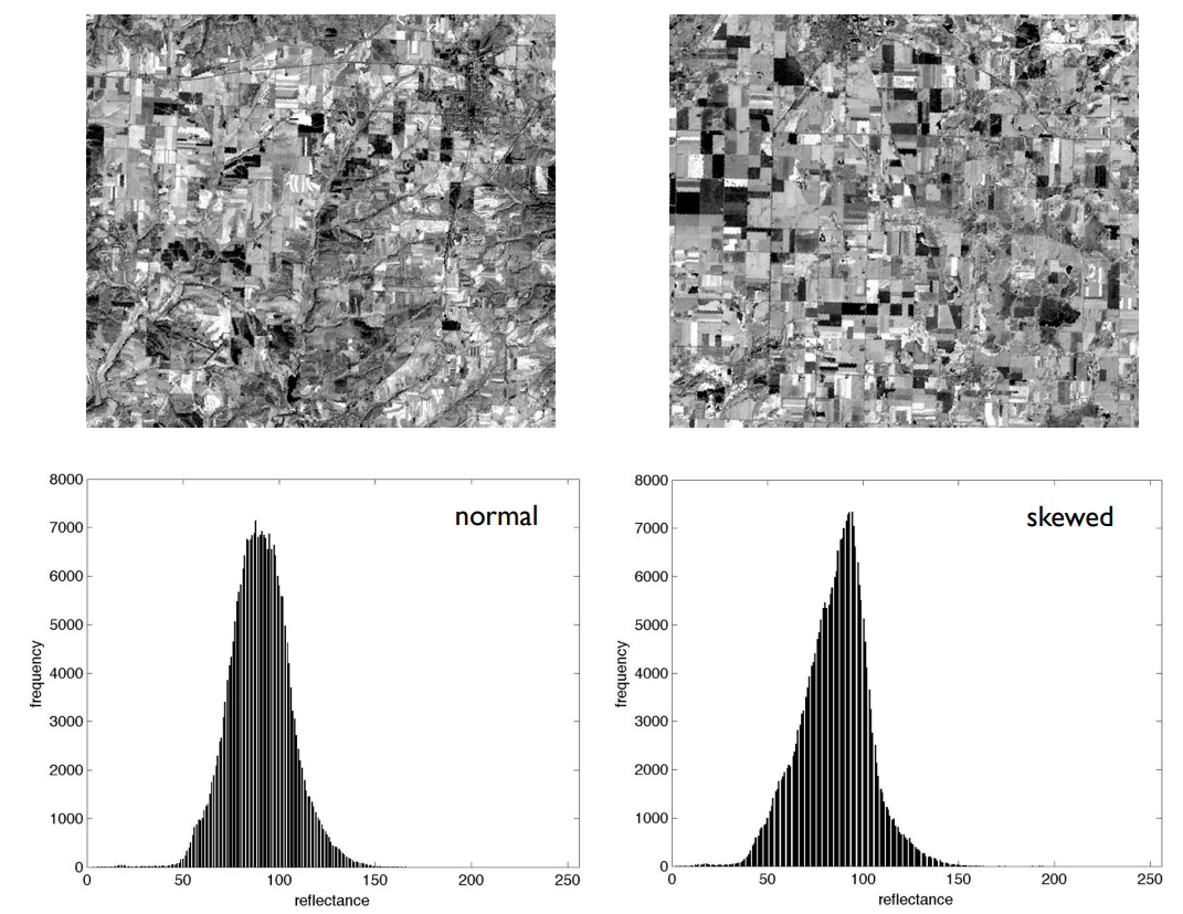
Figure 43: Digital Image histogram. (source: https://lcluc.umd.edu/sites/default/files/lcluc_documents/ozdogan1_lcluc_8-2010_training_0.pdf)

9.3.2.1 Image Enhancements

Contrast Enhancement

The sensor must be able to detect a high dynamic range of values, but one scene in particular has a very low contrast to encompass only limited radiance values. The aim is to improve the visual quality of the image. This will make various transformations (min-max, saturation, equalization, etc.) to the image histogram.

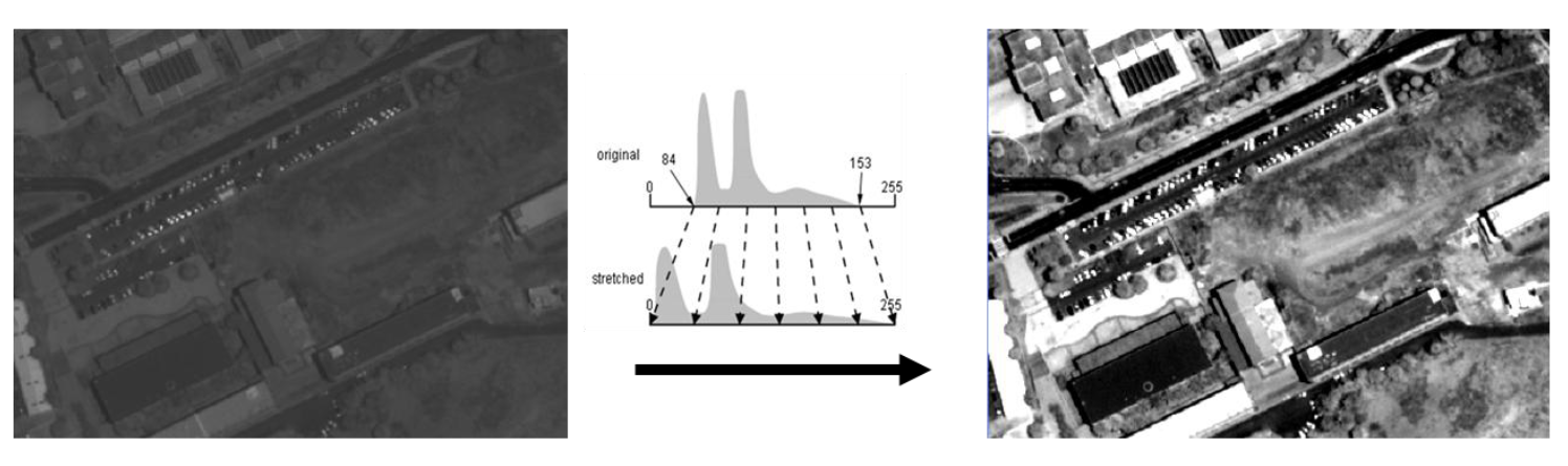
Figure 44: Digital Image Enhancement. (source: Gonzáles et al., 2013)

This involves applying a transformation that maps the original digital levels ($ND$) in gray levels ($NG$):

$NG=T(ND)$.

There are several possibilities of processing levels.These changes are made for each pixel in the image as a separate element and independent of its position in the image using the histogram of the image.

Possible transformations:

linear expansion - Min-Max Stretch expands the dynamic range of the values to fill the full range of reproduction. $GN$: greyscale and $DN$: digital levels. This transformation is sensitive to extreme values (outliers) which can be solved by using of saturation stretch. Same value for all the range could be sensitive to lower symmetric histograms. It can be solved by non-linear stretch or histogram equalization.

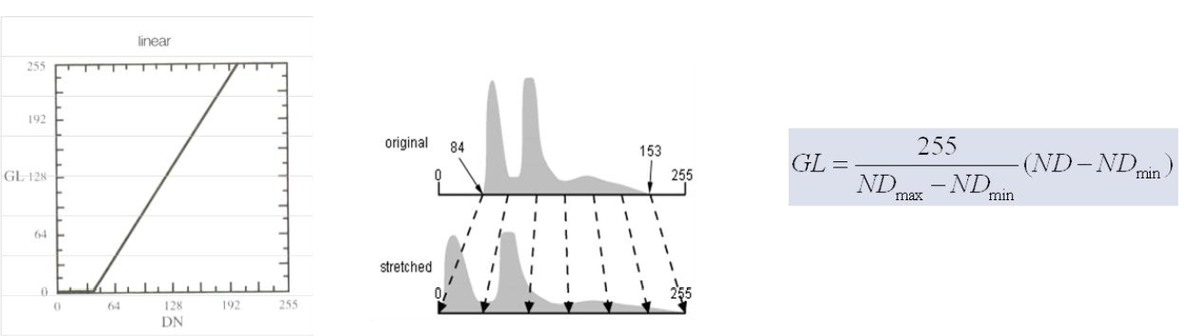
Figure 45: Linear Expansion. (source: Gonzáles et al., 2013)

normalization expansion - robust algorithm (adapted from saturation stretch).It is a linear expansion of a signal with a given mean and variance to cut the ends of the dynamic range. It lets us to control the average value of the output image and to vary the contrast by adjusting the variance.

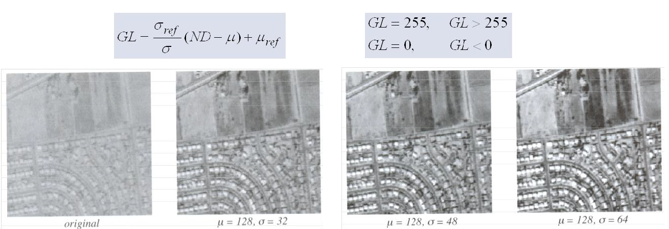Figure 46: Normalization Expansion. (source: Gonzáles et al., 2013) The mean is constant and the contrast varies by changing the variance.

Thresholding - a transformation that classifies the image into two categories (binarized) based on a threshold on the original values of the image. - It requires a greater number of thresholds for a greater number of classes.

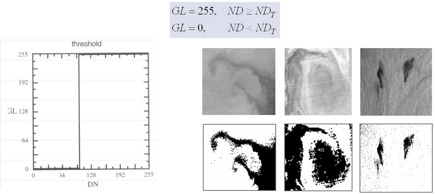
Figure 47: Thresholding. (source: Gonzáles et al., 2013)

Colour Representation

The human eye is more sensitive to colors than gray levels, so it is important the color representation of images for visual analysis. This representation can be done in two ways:

False color representation (Pseudo): when a color table is applied to a grayscale band (LUT: Look-up table) or when red, green or blue colors are assigned to several bands that do not correspond to the true color.
True color representation: when the image is taken by a sensor that captures these 3 bands of color: red, green and blue.

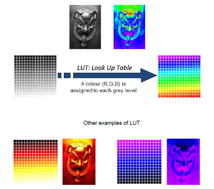
Figure 48: Pseudocolour - one band. (source: Gonzáles et al., 2013)

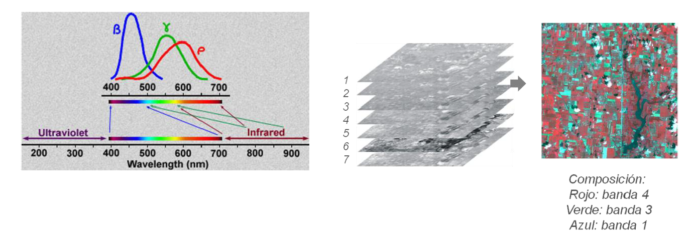
Figure 49: Pseudocolour - multi band. (source: Gonzáles et al., 2013)

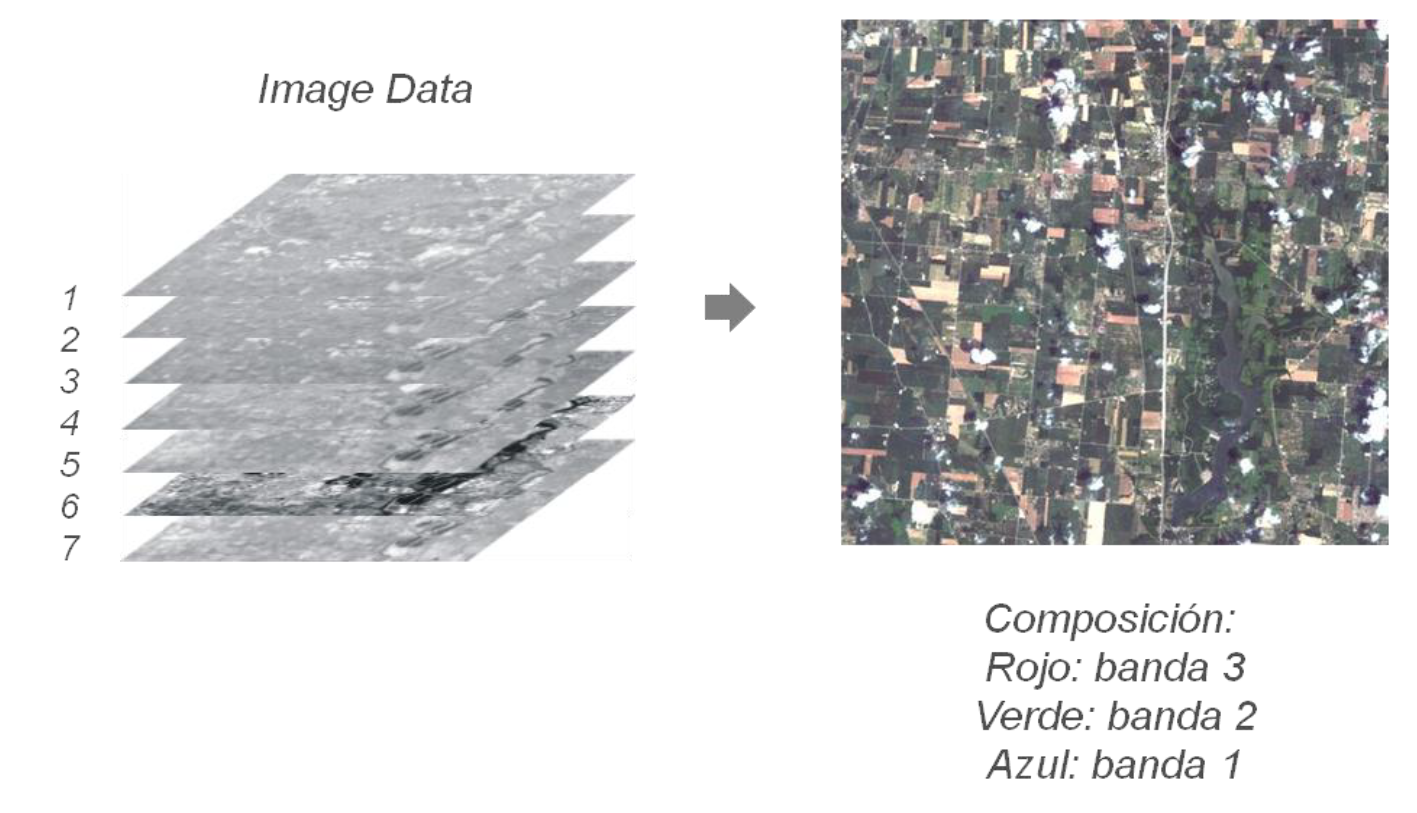
Figure 50: Truecolour. (source: Gonzáles et al., 2013)

Spatial Indexes

They are combinations of bands for obtaining a parameter of interest for classification purposes (vegetation, water, minerals, etc.). They are based on the behavior of the reflectivity parameter to maximize its discrimination:

Vegetation Indexes - they They are mainly based on relations between NIR and R bands. Normalized Difference Vegetation Index (NDVI) is widely used. It generates values between -1 and +1. NDVI is an inaccurate indicator in arid regions.

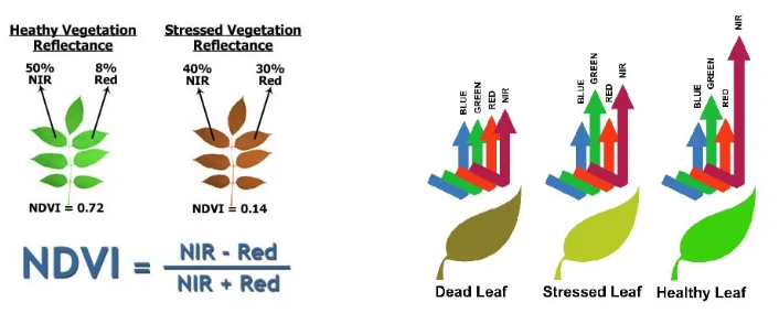
Figure 51: NDVI Principle. (source: https://www.integraldrones.com.au/comparing-ndvi-mapping-systems/)

Convolution Filtering

Technique to modify the spatial information of the image using the digital values of the neighborhood (local filtering).

A window that moves along rows and columns is used.
An operation with the input image’s pixels that fall within the window is carried out and the result is the new pixel of the image in the center position of the window.
It serves for: noise removal/addition, representation of spatial variability of a feature by region, extract particular spatial scale componen from an image, smoothing, edge detection, frequency domain.
By analogy with the procedure used in chemistry to separate components of a suspension, a digital filter is used to extract a particular feature (spatial-scale) component from a digital image.

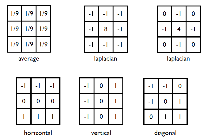
Figure 52: Spatial image enhancements - filtering. (source: https://lcluc.umd.edu/sites/default/files/lcluc_documents/ozdogan1_lcluc_8-2010_training_0.pdf)

9.3.2.2 Image Analysis

Feature Detection

Segmentation is a first step in most image processing problems. It can be defined as finding a partition of the space (Image I) in n disjoint regions to get to satisfy a homogeneity criterion P (.):

$\bigcup\limits_{i=1}^{n} R_{i}=I$

$P(R_{i})=True$

$P(R_{i}\bigcup R_{j}=False)$

The homogeneity criterion can be as simple (or complicated) as desired. Normally, criteria to approach to the semantics of the scene are defined.

This example of coastal upwelling shows the difficulty of segmentation, because objects have no sharp borders and each user may only be interested in a given area and, therefore, each segmentation would be different. As an example, some segmentations obtained by different algorithms are shown in Figure 53.

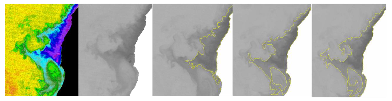
Figure 53: Segmentation example. (source: Gonzáles et al., 2013)

Thematic Classification

It is the step for image analysis that aims at the generation of thematic maps from the input information for the end user. In other words, it tries to transform numerical data into descriptive categories of images to identify the various elements of the image The categories or classes selected for the thematic map should be able to be discriminated from the numerical data of the image.

There are various types of classifiers based on the information used:

Spectral classifier - it is based on the fact that the different classes of the image have different combinations of digital values in each band due to its reflectance or emittance.
Space classifier - it is based on analyzing the relationship between neighboring pixels, considering aspects such as texture, proximity, size, shape, repetition, etc.
Temporal classifier - it uses images on different dates to favor the classification process (e.g., crops or certain types of vegetation have different spectral properties depending on the season which facilitates identification).
Object-oriented classifier - it is a spatial and spectral hybrid classifier which typically includes pipeline stages prior to guide the classification so that each object is assigned entirely to a possible class.

Image Classification Techniques in Remote Sensing

Feature Extraction step (optional)

It is based on applying a spatial or spectral transformation to get the most interesting features for classification.

In this stage:

The information of the image or original bands can be extracted.
Unwanted variability in the spectral signatures (spectral indexes. Example: NDVI in the figure) can be deleted. Spectral separation of classes can be improved.
The number of bands (Principal Component Analysis) can be reduced.

Training step

Select pixels representative of the desired classes to train the classifier. It can be done in a supervised or unsupervised way.

Before jumping to the training phase, it is recommended to analyze the separation of classes to assess a priori whether the classification is possible or if there will be some classes that will not be discriminated.

It is insufficient to only use the distance between the means. It also requires the standard deviation or variance.
Separability measures between classes.

There are several measures of separability from Euclidean and angular distances. Some do not take into account the variance, that is to say, the spectral overlap between the classes, and they become less reliable (in the table there are examples of metric separability).

Supervised Training - training samples are labeled by the user (e.g., figure above). It involves prior knowledge of the terrain (in-situ data, maps, photo interpretation).
Unsupervised Training - training samples are not labeled. Classes are automatically determined.
Mixer Training - it is performed combining both training types. There are several possibilities.

9.3.2.3 Aerial or Satellite Images?

The utility of both satellite images and aerial images as data sources for GIS should be clear by now. Several sources are often available or potentially available for a given study area. An obvious question is “Which should I use?” A number of factors should be considered when selecting an image source.

The image data should provide the necessary spatial resolution. The resolving power of a system depends in part on the difference in color between two adjacent objects, but resolution is generally defined by the smallest high-contrast object that can be detected. Current high-resolution satellite systems have effective spatial resolutions of from one to several meters. Images from mapping cameras, when taken at typical scales and with commonly used film, have maximum resolutions as fine as a few centimeters. Although the gap is narrowing as higher-resolution satellite systems are deployed, aerial images are currently selected in many spatial analyses that require the highest spatial resolution.
The analysis area should be considered. Aerial images are typically less expensive for small areas. Large-scale aerial images are often available from government sources at low cost. Each photograph covers from tens to hundreds of square kilometers, with low cost per square kilometer. As the size of the study area increases, the costs of using aerial photographs may increase. Multi-image mosaics are often needed, raising costs. Terrain distortion may be greater due to poorer geometries. Satellites, because of their high view and larger areal coverage, are less likely to require the creation of mosaics and may have significantly less terrain distortion, important for larger areas.

Satellite scanners may provide a broader spectral range and narrower bands relative to aerial images. As noted earlier, satellite scanners may detect well beyond the visible and near-infrared portions more common in aerial scanners. If important features are best detected using these portions of the spectrum, then satellite data are preferred.

9.4 Airborne LiDAR

A number of laser-based, light detection and ranging systems (LiDAR) are becoming common. Lasers are pointed at the Earth’s surface from an aerial or satellite platform, pulses of laser light emitted, and the reflected energy is recorded (Figure 54). Like radar, laser systems are active because they provide the energy that is sensed. Unlike radar, lasers have limited ability to penetrate clouds, smoke, or haze.

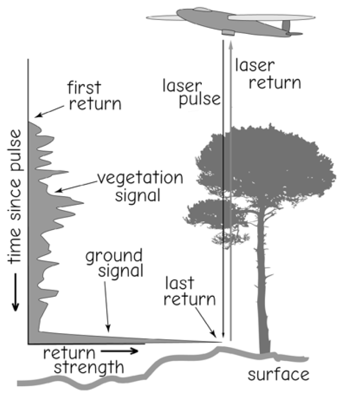
Figure 54: Laser mapping systems operate by generating and then sensing light pulses. The return strength is used to distinguish between vegetation and the ground, and the travel time may be used to determine heights. (source: Bolstad, 2016)

LiDAR systems have been used primarily to gather data about topography, vegetation, and water quality. Laser pulses reflect back from the canopy and the ground, and the strength and timing of the return is used to estimate ground height, canopy height, and other canopy characteristics (Figure 55). LiDAR signals over water also typically result in multiple returns, including water surface height and from various depths, so lasers may be used to measure water clarity and nearshore water depth.

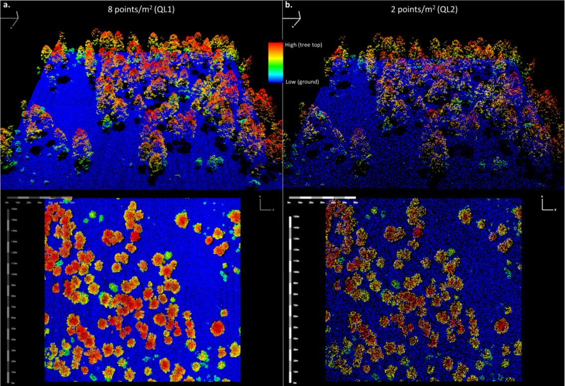
Figure 55: LiDAR point cloud. (source: https://www.usgs.gov/media/images/lidar-point-cloud)

Commercial LiDAR mapping systems are relatively new and have been used primarily for collecting surface data from aircraft and satellites. As noted earlier, three dimensional LiDAR surveying from tripods or ground vehicles is growing, but we’ll not expand on them here.

Aerial LiDAR collection systems typically consist of a downward pointing LiDAR, a precision GNSS to record the plane’s position to a very high accuracy, and an orientation sensing system to measure the angle of the LiDAR pulse relative to the vertical direction. LiDAR energy pulses are directed downward. Some energy from each pulse is reflected from vegetation, buildings, or other features above the ground, but under most conditions many signals reach the ground and return to the airborne laser platform. The time interval between laser pulse emission and the ground return may be used to calculate aircraft height above the terrain. Flying height is known from the GNSS and the terrain elevation calculated for each pulse. Pulses may be sent several thousand times a second, so a trace of ground heights may be measured from every few centimeters to a few meters along the ground.

Discrete-return LiDAR is most common, wherein the system records specific values for each laser pulse downward. Typically the first return from a pulse, last return, and perhaps one to several intermediate returns are recorded. Waveform LiDAR collects a continuous record of the pulse returns, the waveform trace shown in Figure 54.

Discrete-return LiDAR systems produce point clouds, consisting of X, Y, and Z coordinates (Figure 55), and the intensity, scan angle, return order, and other information. Modern laser systems often produce densities of several to tens of points per square meter of ground area, and these point clouds must be processed to remove errors, identify ground points, and assign points to feature types such as buildings or vegetation. Software for primary processing has been developed by most vendors, so that files are delivered with the coordinate and height data assigned to the highest practical accuracy, and points classified with a standard number code that indicates the type of feature “hit by,” or associated with each laser return. These standard codes identify ground (value = 2), buildings (value = 6), or water (value =9). Several characteristics are used to classify points by feature type, including return strength, point order (first, last, or intermediate), local slope or texture, and the location and strength of adjacent returns.

There are a growing number of statewide LiDAR projects, often driven by floodplain mapping or for improved topographic measurements. Ground resolutions of 10 cm (4 in) or better are currently possible when LiDAR is combined with precise GNSS and aircraft orientation measurements. These projects report the “average” point density, but LiDAR returns are typically collected in swaths across the landscape, with individual scan lines discernible when viewed at large scales (Figure 6-39). Projects are planned and flown such that an appropriate amount of overlap exists between adjacent scans and adjacent flight paths, both to avoid gaps in coverage and areas with an unacceptably low sampling density.

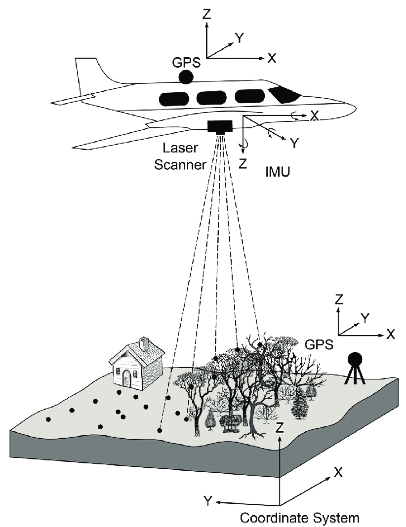
Figure 56: Typical airborne laser scanning system. (source: https://www.researchgate.net/figure/Typical-airborne-laser-scanning-system_fig6_315797574)

Processing extracts the most relevant return for the desired product, for example, the maximum first return in a given square area may be extracted and assigned to a raster cell when calculating tree height, or a mean or minimum value when extracting ground heights. Different processing of the LiDAR point cloud will result in different extracted values.

Horizontal and vertical errors less than a few centimeters are attainable, allowing the use of airborne lasers to measure building height (Figure 57), floodplain location and extent, and slope and derived terrain characteristics, at much higher density and accuracy, over large areas, than previously possible.

LiDAR data have also been widely used to estimate vegetation characteristics, including tree height, forest density, forest wood amounts, growth rates, and forest type. A large number of points reach the ground in all but the densest forests, and the ground vs. locally highest canopy returns usually give an estimate of tree height that is as accurate as traditional manual measurements. The proportion of LiDAR returns is strongly related to canopy density, and to tree and forest wood mass. Crown shape can be determined from dense LiDAR data, which in turn helps separate forest types.

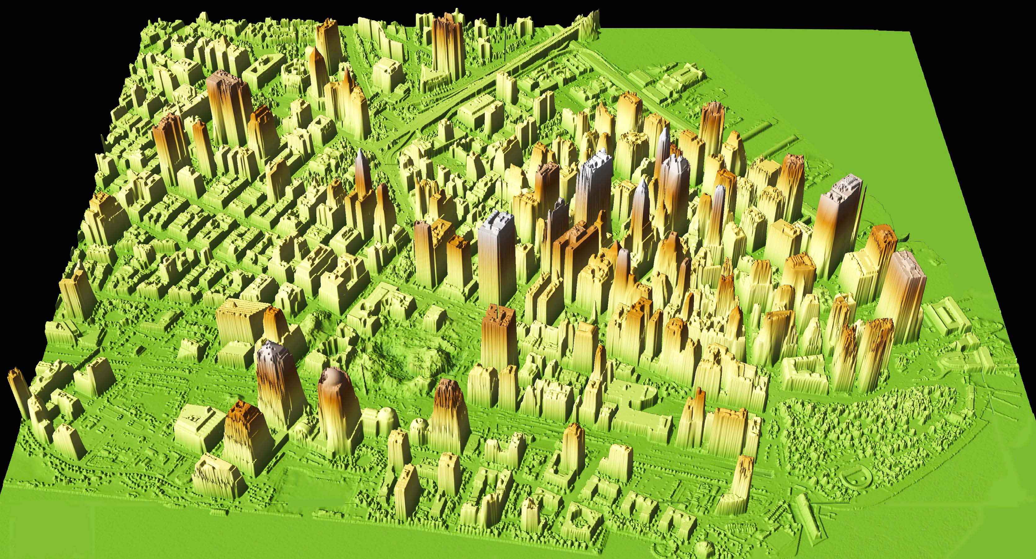
Figure 57: An example of LiDARdata and depiction of building heights. This image shows lower Manhattan, New York in late 2001. Tallest buildings are shown in white, and the land and water surfaces in green (courtesy NASA). (source: Bolstad, 2016)

There is a standard LAS format, maintained by the American Society of Photogrammetry and Remote Sensing (ASPRS). The standard defines the file structure, content, storage order, naming, codes, and all other information so that any user may be able to access, process, and distribute LiDAR data in a standard way. The standard has evolved through various versions, up to 1.3 when this book edition was written. The convention defines the standard LiDAR exchange file with a .las file extension, for example, mylidar.las. Also note that there are competing, nonstandard, compressed formats defined by some providers, for example, ESRI supports their own “optimized” LAS format, and rapidlasso also has specified a compressed format. Neither are guaranteed to be compatible with standard ASPRS files. Caution should be exercised when using nonstandard file formats, and the formats should at a minimum be openly defined, with all users having access to the file and storage specifications, and the ability to write independent code to read and write the files.

9.5 Small Unmanned Aerial Vehicles: Drones

Small, unmanned planes and helicopters have been introduced over the past decade to collect data for GIS (Figure 58). Variously called unmanned aerial vehicles (UAVs), remotely piloted vehicles (RPV), or simply drones, they may substantially reduce the cost and increase the flexibility of data collection. Data may also require increased processing times and exhibit more variable accuracy, given the small footprint and greater difficulty maintaining a level orientation in these small aircraft. However, almost all of the previous descriptions of image and LiDAR data systems and processing apply to data collected from drones because they typically carry small versions of cameras, LiDARs, and other detectors.

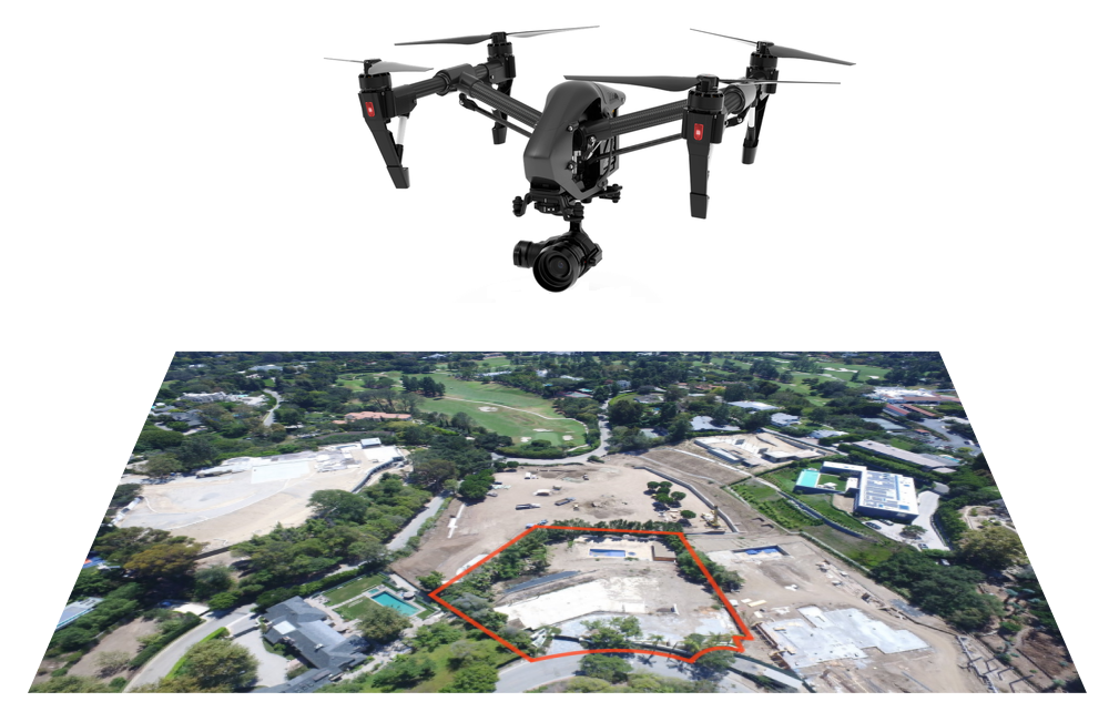
Figure 58: Drone mapping. (source: https://beverlyhillsaerials.com/mapping/)

One primary advantage of drones is low cost and ease of deployment. Many drone systems for GIS data collection currently cost less than $100,000, and some for below $10,000, including all subsystems and software for converting raw images into georeferenced 2D and 3D registered images. Drones may be carried to a site and launched, often by hand for the smallest units, using preprogrammed flight lines to collect images along a specified path. This allows data collection at the time and place of interest, provided weather and other conditions are apt. Smaller data collection windows may be utilized, increasing the likelihood of data acquisition.

High data resolutions may be another advantage of UAVs. Because they may be flown at low altitudes, pixel sizes of a few centimeters or less are possible. Individual bridge beams, rooftop fans, or paths may be resolved, leading to more detailed data, with very high point densities.

Smaller UAVs are limited in their data collection rates, and likely will not be suitable for areas much larger than a few square kilometers. They fly at relatively low speeds, and typically carry small camera systems with commensurately small image footprints. UAVs for GIS data collection range in size from less than a meter wingspan through several to tens of meters, and there is a trade-off, with increasing costs associated with increasing system throughput. Larger UAVs may collect data at rates approaching current manned aerial systems, but in doing so lose many of the cost, flexibility, and resolution advantages.

Spatial data from small UAVs may be of more variable quality than that from traditional flow platforms. Camera systems are typically not as specialized on UAVs, with greater spherical and other lens distortion, less accurate GNSS and hence potentially larger positioning errors, and more dependent on less well-trained operators or analysts. Many of these potential limitations may be addressed in appropriately developed software, for example, image correlation and 3D reconstruction algorithms may be robust in finding a correct solution, and advising the analysts when they are unable to reach acceptable accuracies. Lens or other system distortions may be removed through precise calibration using standardized test patterns, but these measures are not guaranteed for all presently available UAV systems marketed as spatial data collection tools. It is up to the data consumer to verify the proclaimed accuracy of any system.

Finally, there is substantial regulatory uncertainty regarding UAV operation. Given that millions of UAVs will likely be deployed over the next few years, many by hobbyists, there are real risks to civilian passenger aviation. This, plus perceived invasion of privacy concerns, make it likely that UAV operation may require licensing or become restricted.

More about Drones - look at these sources:

9.5.1 Summary

Aerial and satellite images are valuable sources of spatial data. Photos and images provide large-area coverage, geometric accuracy, and a permanent record of spatial and attribute data, and techniques have been well developed for their use as a data source. Remote sensing is based on differences among features in the amount of reflected electromagnetic energy. Chemical or electronic sensors record the amount of energy reflected from objects. Reflectance differences are the basis for images, which may in turn be interpreted to provide information on the type and location of important features.

Aerial images are a primary source of coordinate and attribute data. Camera-based mapping systems are well developed, and are the basis for most large-scale topographic maps currently in use. Camera tilt and terrain variation may cause large errors on aerial images; however, methods have been developed for the removal of these errors. Terrain-caused image displacement is the basis for stereophotographic determination of elevations.

Satellite images are available from a range of sources and for a number of specific purposes. Landsat, the first land remote sensing system, has been in operation for nearly 30 years, and has demonstrated the utility of satellite images. SPOT, AVHRR, Ikonos, and other satellite systems have been developed that provide a range of spatial, spectral, and temporal resolutions.

Aerial and satellite images often must be interpreted to provide useful spatial information. Aerial images are typically interpreted manually. An analyst identifies features based on their shape, size, texture, location, color, and brightness, and draws boundaries or locations, either on a hardcopy overlay, or on a scanned image. Satellite images are often interpreted using automated or semiautomated methods. Classification is a common interpretation technique that involves specifying spectral and perhaps spatial characteristics common to each feature type.

The choice of photographs or satellite imagery depends on the needs and budgets of the user. Aerial images often provide more detail, are less expensive, and are easily and inexpensively interpreted for small areas. Satellite images cover large areas in a uniform manner, and sense energy across a broader range of wavelengths. LiDAR data are becoming a widespread source of spatial data. Discrete-return LiDAR are prevalent, providing X, Y, and Z coordinates for ground and above-ground feature returns. Most new, high-resolution digital elevation models are based on LiDAR data, and building and forest features are routinely extracted from LiDAR. Statewide acquisitions are becoming common, and system resolution and collection frequency are likely to improve through time.

Unmanned aerial vehicles (UAVs), also known as drones, show promise as spatial data collection tools. Lower costs, increased flexibility, and higher details must be weighed against limitations in throughput and hence area imaged, variability in accuracy, and regulatory uncertainty.

Satellite Maps

25 Satellite Maps To See Earth in New Ways (2020)

Literature:

González, F., E., Ruiz, M. J., and Acosta, F.,M. (2013): Remote Sensing Tutorial. 337 pp., Universidad de las Palmas de Gran Canaria.
Konecny, G. (2014): Geoinformation: Remote Sensing, Photogrammetry and Geographic Information Systems.
Linder, W.(2016): Digital Photogrammetry: A Practical Course. 223 pp., Springer.
Wolf, P., R., Dewit, B., A. and Wilkinson, B., E.(2014): Elements of Photogrammetry: With Applications in GIS. 663 pp., McGraw-Hill Education.

Another recommended source for those interested:

Data