11 Vector data analysis

Because points, lines and areas are so different from one another, the type of queries they are used for and hence the algorithms developed for them, are sometimes different. Some queries are just not meaningful for all vector types. For example, polygons can contain points but points cannot contain polygons, so a point in polygon test is useful but polygon in point test is not. Even queries are meaningful for all types, they may need to work rather differently. For instance, it is possible to measure the distance between any two features. If both are points, this is simple, but if they are areas, then there are several possible distances: the distance between the nearest points on the boundaries, the distance between centroids (Wise, 2002).

Most fundamental vector algorithms are chosen in this chapter.

11.1 Length and area for vector data

Since the majority of GIS mapping involves the use of datasets that are provided in projected, plane coordinates, distances and associated operations such as area calculations are carried out using Euclidean geometry. Polygon areas (and the areas of sections of polygons) are calculated using integration by the trapezoidal or Simpson’s rule, taking advantage of the fact that progressing clockwise around all the polygon vertices generates the desired result.

For example, in Figure 1 the area between the x-axis and the two vertical lines at \(x_1\) and \(x_2\) is simply the width between the two lines, i.e. (\(x_2‑x_1\)) times the average height of the two verticals, i.e. \((y_1+y_2)/2\), giving a rectangle like the first one shown to the right of the polygon. Thus this rectangle has area:

\(A_i=\frac{1}{2}(x_2-x_1)(y_1+y_2)\qquad\qquad (1)\).

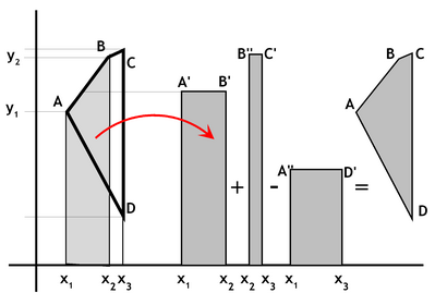
Figure 1: Area calculation using Simpson´s rule. (source: https://www.spatialanalysisonline.com/)

The area between the \(x\)-axis and the two verticals at \(x_2\) and \(x_3\) is shown by the second narrow rectangle, and if we then subtract the shorter and wider rectangle, which represents the area outside of the polygon between the two vertical lines of interest, we obtain the area of the part of the overall polygon we are interested in (\(A,B,C,D\)). More generally, if we take the (\(n‑1\)) distinct coordinates of the polygon vertices to be the set \(\{x_i,y_i\}\) with \((x_n,y_n)=(x_1,y_1)\) then the total area of the polygon is given by:

\(A=\sum\limits_{i=1}^{n-1}\frac{1}{2}(x_2-x_1)(y_1+y_2)\qquad\qquad (2)\).

This is an expression we use also in connection with the determination of polygon centroids. If the order is reversed the total is the same but has a negative sign. This feature can be used to remove unwanted polygons contained within the main polygon (e.g. areas of water or built-up zones within a district when calculating available land area for farming or the area to be included and excluded in density or similar areal computations). The procedure fails if the polygon is self-crossing (which should not occur in well-structure GIS files) or if some of the y‑coordinates are negative — in this latter case either positive-only coordinate systems should be used or a fixed value added (temporarily) to all \(y\)-coordinate values to ensure they all remain positive during the calculation process.

Lengths and areas are normally computed using Cartesian (\(x,y\)) coordinates, which is satisfactory for most purposes where small regions (under 100 kms x 100 kms) are involved. For larger areas, such as entire countries or continents, and where data are stored and manipulated in latitude/longitude form, lengths (distances) and areas should be computed using spherical or similar measures (e.g. ellipsoidal, geoidal). If one uses Cartesian calculations over large regions the results will be incorrect — for example, using the standard ArcGIS measure tool to show the distance between Cairo and Capetown on a map of Africa will give a value substantially different from the “true”, great circle distance (depending on the projection applied in ArcGIS). Computation of polygon areas using spherical or ellipsoidal models is complex, requiring careful numerical integration.

In some cases GIS software products will select the appropriate calculation method based on the dataset, whilst in others (e.g. MapInfo) the option to specify Cartesian or Spherical computation may be provided where relevant. If we identify two mapped locations as having Cartesian coordinates (\(x_i,y_i\)) and (\(x_j,y_j\)) then the distance between them, \(d_{ij}\), is simply the familiar:

\(d_{ij}=\sqrt{(x_i-x_j)^2+(y_i-y_j)^2})\qquad\qquad (3)\).

A straight line, \(l\), in the \(x-y\) plane can be expressed as an equation: \(ax+by+c=0\), where \(a, b\) and \(c\) are constants. Using this formulation the Euclidean distance of a point \(p(x_p,y_p)\) from this line is given by (Figure 2):

\(d_{p,l}=\frac{|ax_p+by_p+c|}{\sqrt{a^2+b^2}}\qquad\qquad (4)\).

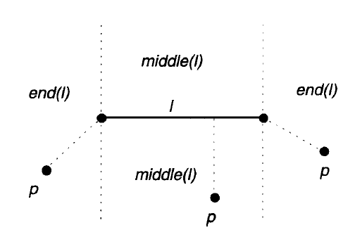
Figure 2: Distance between a point and line segment (source: Worboys, 2003)

The problem becomes more complex for a polyline, as can be seen from Figure 3. For each segment \(l\), it must be checked whether \(p\) lies in middle(\(l\)) and if so the distance calculated. The distance from \(p\) to each vertex is also calculated. The distance of \(p\) from the chain will be the minimum of all these distances. If the number of segments in the chain is \(n\), then the time complexity of the computation is \(O(n)\). An approximation to the distance may be achieved by considering only the distances to vertices of the chain. This approximation will be good in general if the segment lengths are small compared with the distance of the point from the chain.

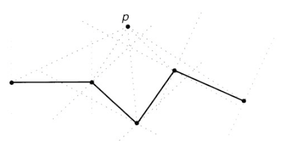
Figure 3: Distance between a point and line segment (source: Worboys, 2003)

Distances from a point to a polygon or between polygons may be required in terms of their boundaries. Thus, the distance between two polygons may be interpreted as the distance between their closest points. In that case, a calculation involving boundary polylines may be necessary. More usually, the distance between two polygons is interpreted as the distance between their centroids. This leads to the next section, where the calculation of the centroid of a polygonal area is discussed.

GIS the distance from a point to a line segment or set of line segments (e.g. a polyline) is frequently needed. This requires computation of one of three possible distances for each (point, line segment) pair:

1. if a line can be extended from the sample point that is orthogonal to the line segment, then the distance can be computed using the general formula \(d_{p,l}\) provided above (equation 4);
2. (equation 5) and c) (equation 6) if case 1. does not apply, the sample point must lie in a position that means the closest point of the line segment is one of its two end points. The minimum of these two is taken in this instance. The process is then repeated for each part of the polyline and the minimum of all the lengths computed selected.

In spherical coordinates the (great circle) distance equation often quoted is the so-called Cosine formula:

\(d_{ij}=R\cos^{-1}[\sin \phi_i \sin\phi_j +\cos\phi_i\cos\phi_j\cos (\lambda_i\lambda_j)]\qquad\qquad (5)\),

where: \(R\) is the radius of the Earth (e.g. the average radius of the WGS84 ellipsoid); (\(φ,λ\)) pairs are the latitude and longitude values for the points under consideration; and \(‑180≤λ≤180\), \(‑90≤φ≤90\) (in degrees, although such calculations normally are computed using radians; n.b.\(180^o=1 \ rad\) and \(1\ rad\doteq 57.30^o\)). This formula is sensitive to computational errors in some instances (very small angular differences). A safer equation to use is the Haversine formula:

\(d_{ij}=2R\sin^{-1}\left(\sqrt{\sin^2 A+\sin^2 B\cos\phi_i\cos\phi_j}\right)\qquad\qquad (6)\),

where: \(A=\frac{\phi_i-\phi_j}{2}, B=\frac{\lambda_i-\lambda_j}{2}\).

Most GIS packages do not specify how they carry out such operations, although in many cases basic computations are made using the Euclidean metric and reported in decimal degrees. Distances calculated using the Haversine formula we shall denote \(d_S\), or Spherical distance (Figure 4).

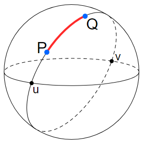
Figure 4: Spherical distance (source: https://en.wikipedia.org/wiki/Great-circle_distance)

11.2 Surface area

11.2.1 Projected surfaces

Most GIS packages report planar area, not surface area. Some packages, such as ArcGIS (3D Analyst) and Surfer provide the option to compute surface area. Computation of surface areas will result in a value that is greater than or equal to the equivalent planar projection of the surface. The ratio between the two values provides a crude index of surface roughness.

If a surface is represented in TIN form, the surface area is simply the sum of the areas of the triangular elements that make up the TIN. Let \(T_j=[x_{ij},y_{ij},z_{ij}],\ i=1,2,3\) be the coordinates of the corner points of the \(j\)th TIN element. Then the surface area of the planar triangulation (or planimetric area) determined when \(z\)=constant, can be calculated from a series of simple cross-products:

\(A_{j}=\frac{1}{2}\left(\begin{array}{c} +x_{2j}y_{1j}+x_{3j}y_{2j}+x_{1j}y_{3j}\\ -x_{1j}y_{2j}-x_{2j}y_{3j}-x_{3j}y_{1j}\\ \end{array}\right)\qquad\qquad (7)\).

Note that this expression is the same as the polygon area formula we provided earlier, but for a (\(n‑1\))=3‑vertex polygon:

\(A=\frac{1}{2}\sum\limits_{i=1}^3 (x_{i+1}y_i-x_iy_{i+1})\qquad\qquad (8)\),

where \(i+1=4\) is defined as the first point, \(i=1\). The term inside the brackets is the entire area of a parallelogram, and half this gives us our triangle area. This expression can also be written in a convenient matrix determinant form (ignoring the \(j\)’s for now) as:

\(A=-\frac{1}{2}\left|\begin{array}{ccc} x_1 & y_1 & 1\\ x_2 & y_2 & 1\\ x_3 & y_3 & 1\\ \end{array}\right|\qquad\qquad (9)\).

If the slope of \(T_j, θ_j\), is already known or easily computed, the area of \(T_j\) can be directly estimated as \(A_j/cos(θ_j)\) (Figure 5). Alternatively the three dimensional equivalent of the matrix expression above can be written in a similar form, as:

\(A=\frac{1}{2}\sqrt{\left|\begin{array}{ccc} x_1 & y_1 & 1 \\ x_2 & y_2 & 1 \\ x_3 & y_3 & 1 \\ \end{array} \right|^{2}+\left|\begin{array}{ccc} y_1 & z_1 & 1 \\ y_2 & z_2 & 1 \\ y_3 & z_3 & 1 \\ \end{array} \right|^{2}+\left|\begin{array}{ccc} z_1 & x_1 & 1 \\ z_2 & x_2 & 1 \\ z_3 & x_3 & 1 \\ \end{array} \right|^{2}}\qquad\qquad (10)\).

If \(z=0\) for all \(i\), the second and third terms in this expression disappear and we are left with the result for the plane. Suppose that we have a plane right angled triangle with sides 1,1 and \(\sqrt{2}\), defined by the 3D coordinates: \((0,0,0), (1,0,0)\) and \((1,1,0)\). This plane triangle has area of one half of a square of side length 1, so its area is 0.5 units, as can be confirmed using the first formula above. If we now set one corner, say the point \((1,1,0)\) to have a \(z\)-value (height) of 1, its coordinate becomes \((1,1,1)\) and the area increases to 0.7071 units, i.e. by around 40%.

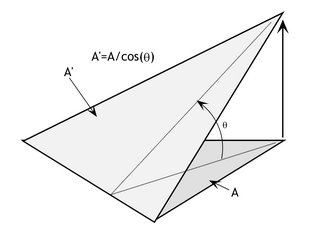
Figure 5: Planimetric and surface area of a 3D triangle (source: https://www.spatialanalysisonline.com/HTML/index.html)

If the surface representation is not in TIN form, but represented as a grid or DEM, surface area can again be computed by TIN-like computations. In this case the 8-position immediate neighborhood of each cell can be remapped as a set of 8 triangles connecting the center-points of each cell to the target cell. Connecting all cell centers in this way creates a form of TIN and surface computation proceeds as described above – this is the procedure used in ArcGIS (3D Analyst). A more sophisticated method involves a similar form of computation but calculated on a cell-by-cell weighted basis. In this procedure the surface area for each cell is taken as a weighted sum of eight small triangular areas. The area of triangles centered on the target cell are computed and 25% of each such area is assigned to the central cell (shaded gray in Figure 6B).

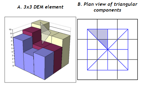
Figure 6: DEM surface area (source: https://www.spatialanalysisonline.com/HTML/index.html)

Research has suggested that the resulting total surface area for the cell is close to that produced by TIN models for grids of 250+ cells. We can examine this model more closely by taking a specific example. Let us assume that the 3x3 DEM surface segment in Figure 6 has cells which are 1 meter square and elevation values given in meters as shown below:

\(\begin{array}{ccc} 10 & 8 & 8 \\ 9 & 6 & 6 \\ 8 & 5 & 6 \\ \end{array}\)

The nine individual cells can be referenced in various ways – below use a simple numerical referencing around the central or target cell:

\(\begin{array}{ccc} 1 & 2 & 3 \\ 8 & 0 & 4 \\ 7 & 6 & 5 \\ \end{array}\)

The planar area of each cell is simply 1x1, so 1 square meter. To compute the estimated surface area we need to calculate the area of each of the 8 sloping triangles and allocate 25% of this area to the central cell. To do this we use the determinant expression shown earlier. For the triangle shown in Figure 6A (the triangle connecting cells 1-2-0) this gives an area of 3/2, so 25% of this gives 3/8 units as opposed to the 1/8 units that to a flat triangle such as 0-4-5. Continuing this computation for all 8 triangles gives the overall estimated surface area using this algorithm as 2.5 sq.m. The process is then repeated for every pixel, adjusting for edge effects where necessary as with many other operations of this type (e.g. by adding a temporary row or column to each edge that duplicates the existing values).

This example is unrealistic of course since in most DEM datasets the horizontal and vertical scales are not the same. For example, if the individual cell sizes in the example above are 10 meters x 10 meters and the vertical measurements are in meters, the procedure yields a surface area approximately 3% greater than the planar area. Grid surface areas can also be computed using the slope adjustment method described above assuming that a slope grid has been first been computed, or using grid data with linear interpolation to facilitate simpler 3D quadrilateral computations.

Surface areas are computed relative to a reference plane, usually z=zmin or z=0. In some instances it may be necessary to specify the value to be associated with the reference plane, and whether the absolute values, positive values and/or negative values are to be computed. Surfer, for example, supports all three options which it describes as positive planar and surface area, negative planar and surface area and total planar and surface area. For example, consider the surface illustrated in Figure 7. This shows a surface model of a GB Ordnance Survey DEM for tile TQ81NE, which we shall use as a test surface in various sections of this Guide. This is a 5,000 m x 5,000 m area provided as a 10 m x 10 m grid of elevations, with an elevation range from around 10 m ‑ 70 m. Using a reference plane of z=30m the surface area above this reference plane is roughly 1.3sq kms and below 30 m is roughly 2.1sq kms (3.4sq kms in total compared to 2.5sq kms for the planar area).

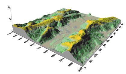
Figure 7: Surface model of DEM (source: https://www.spatialanalysisonline.com/HTML/index.html)

11.2.2 Terrestrial (unprojected) surface area

For large regions (e.g. “rectangular” regions with sides greater than several hundred kilometers) surface areas will be noticeably affected by the curvature of the Earth. Such computations apply at large State and continental levels, or where the areas of ocean, ice or cloud cover are required over large regions. Computation of areas using spherical trigonometry or numerical integration is preferable in such cases.

The area of a spherical rectangular region defined by fixed latitude and longitude coordinates is greater than the area bounded by lines of constant latitude — the latter are not great circles, although the lines of longitude are. This effect increases rapidly nearer the poles and is weakest close to the equator. The MATLab Mapping Toolbox (MMT) function AREAQUAD provides a convenient way of computing the area of a latitude-longitude “quadrangle”, although it can be computed without too much difficulty using spherical trigonometry. The area north of a line of latitude, \(φ\), is the key factor in the calculation (the surface area of an entire sphere is \(4πR^2\)). The former area is:

\(A=2\pi (1-\sin \varphi)R^2\qquad\qquad (11)\),

where \(R\) is the radius of the spherical Earth, e.g. 6378.137 kms. The area of the quadrangle is then simply the difference between the areas, \(A_1\) and \(A_2\), north of each of the two lines of latitude, \(φ_1\) and \(φ_2\), adjusted by the proportion of the Earth included in the difference in longitude values, \(λ_1\) and \(λ_2\):

\(A=\frac{\pi}{180}|A_1-A_2||\lambda_1-\lambda_2|R^{2}\qquad\qquad (12)\).

A (simple) polygon with \(n\) vertices on the surface of the Earth has sides that are great circles and area:

\(A=\left( \sum\limits_i \theta -(n-2)\pi \right)R^2\qquad\qquad (13)\),

where again \(R\) is the radius of the Earth and the \(θ_i\) are the internal angles of the polygon in radians measured at each polygon vertex. The simplest spherical polygon is a triangle (\(n=3\) so \(n‑2=1\)) and on a sphere the sum of its internal angles must be greater than 180 degrees (\(\pi\)), so the formula equates to 0 when the triangle is vanishingly small. A spherical triangle with internal angles that are all 180 degrees is the largest possible, and is itself a great circle. In this case the formula yields \(A=2πR^2\), as expected.

All polygon arcs must be represented by great circles and internal angles are to be measured with respect to these curved arcs. The term in brackets is sometimes known as the spherical excess and denoted with the letter \(E\), thus \(A=ER^2\). Note that every simple polygon on a sphere divides it into two sections, one smaller than the other unless all vertices lie on a great circle. If only the latitude and longitude values are known, the internal angles must be computed by calculating the true great circle bearing (or azimuth) from each vertex to the next — this can be achieved using spherical trigonometry or, for example, the MMT function AZIMUTH, which supports explicit geoid values. Azimuth values are reported from due north, so computations of internal angles need to adjust for this factor. Alternatively the MMT function AREAINT may be used, ideally with high point density (i.e. introducing additional vertices along the polygon arcs). This latter function computes the enclosed area numerically. The open source GIS, GRASS, provides a number of similar functions, including the source code modules area_poly1, which computes polygon areas on an ellipsoid where connecting lines are grid lines rather than great circles, and area_poly2 which computes planimetric polygon area.

11.3 Line Smoothing and point-weeding

Polylines and polygons that have a large number of segments may be considered over-complex or poor representations of the original features, or unsuitable for display and printing at all map scales (a problem of map generalization). A range of procedures exist to achieve simplification of lines in such cases, including those illustrated in Figure 8.

11.3.1 Point weeding

Point weeding is a procedure largely due to Douglas and Peuker (1973) — for a fuller discussion, see Whyatt and Wade (1988) and Visvalingam and Whyatt (1991). In the example shown in Figure 8A the original black line connecting all the vertices 1 to 10 is progressively simplified to form the dotted (green) line shown. The procedure commences by connecting point 1 (the anchor) to point 10 (the floating point) with a temporary line (the initial segment). This enables point 8 to be identified as the vertex that deviates from this initial segment by the greatest distance (and more than a user-defined tolerance level, shown here by the bar symbol on the left of the upper diagram). Euclidean distance squared is sufficient for this algorithm and is significantly faster to compute. Point 10 is then directly connected to point 8 and point 9 is dropped. A new temporary line is drawn between point 8 (the new floating point) and 1 and the process is repeated. This time points 5, 6 and 7 are dropped. Finally point 3 is dropped and the final line contains only 4 segments and 5 nodes (1, 2, 4, 8 and 10).

This process can be iterated by moving the initial anchor point to the previous floating point and repeating the process for further simplification. Some implementations of this algorithm, including those of the original authors, fail to handle exceptions where the furthest point from the initial segment is one end of a line that itself lies close to the initial segment. Ebisch (2002) addresses this error and provides corrected code for the procedure. The procedure is very sensitive to the tolerance value selected, with larger values resulting in elimination of more intermediate points.

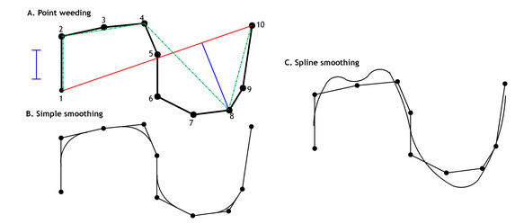
Figure 8: Smoothing techniques (source: https://www.spatialanalysisonline.com/HTML/index.html)

A number of GIS products provide a range of simplification methods. The default in ArcGIS is point-weeding (POINT_REMOVE) but an alternative BEND_SIMPLIFY which removes extraneous bends is also available.

11.3.2 Simple smoothing

Simple smoothing utilizes a family of procedures in which the set of points is replaced by a smooth line consisting of a set of curves and straight line segments, closely following but not necessarily passing through the nodes of the original polyline. This may be achieved in many ways with Figure 8B showing one example.

11.3.3 Spline smoothing

This method typically involves replacing the original polyline with a curve that passes through the nodes of the polyline but does not necessarily align with it anywhere else, or approximates the point set rather like a regression fit (Figure 8c). A range of spline functions and modes of operation are available (including in some cases Bézier curves and their extension, B-splines), many of which involve using a series of smoothly connected cubic curves. In some cases additional temporary nodes or “knots” are introduced (e.g. half way between each existing vertex) to force the spline function to remain close to the original polyline form.

Each method and implementation (including the selection of parameters and constraints for each variant) will have different results within and across different GIS packages and the process will not generally be reversible. Furthermore, different GIS packages tend to offer only one or two smoothing procedures, so obtaining consistent results across implementations is almost impossible. Note that once a polyline or polygon has been subject to smoothing its length will be altered, becoming shorter in many cases, and enclosed areas will also be altered though generally by a lesser amount in percentage terms. The orientation of the line segments also changes dramatically, but not the relative positions of the two end nodes, so the end-node to end-node orientation is retained. Determination of the length and area of amended features may require numerical integration utilizing fine division of the smoothed objects rather than the simple procedures we have described above.

11.4 Centroid of a polygon

The terms center and centroid have a variety of different meanings and formulas, depending on the writer and/or software package in which they are implemented. There are also specific measures used for polygons, point sets and lines so we treat each separately below. Centers or centroids are provided in many GIS packages for multiple polygons and/or lines, and in such cases the combined location is typically computed in the same manner as for point sets, using the centers or centroids of the individual objects as the input points. In almost all cases the metric utilized is \(d_E\) or \(d_S\), although other metrics may be more appropriate for some problems.

Centroids are often defined as the nominal center of gravity for an object or collection of objects, but many other measures of centrality are commonly employed within GIS and related packages. In these latter instances the term center (qualified where necessary by how this center has been determined) is more appropriate than centroid, the latter being a term that should be reserved for the center of gravity.

11.4.1 Polygon centroids and centers

Polygon centers have many important functions in GIS: they are sometimes used as “handle points”, by which an object may be selected, moved or rotated; they may be the default position for labeling; and for analytical purposes they are often used to “represent” the polygon, for example in distance calculations (zone to zone) and when assigning zone attribute values to a point location (e.g. income per capita, disease incidence, soil composition). The effect of such assignment is to assume that the variable of interest is well approximated by assigning values to a single point, which essentially involves loss of information. This is satisfactory for some problems, especially where the polygons are small, homogeneous and relatively compact (e.g. unit ZIP-code or postcode areas, residential land parcels), but in other cases warrants closer examination.

With a number of raster-based GIS packages the process of vector file importing may utilize polygon centers as an alternative to the polygons themselves, applying interpolation to the values at these centroids in order to create a continuously varying grid rather than the common procedure of creating a gridded version of discretely classified polygonal areas. Similar procedures may be applied in vector-based systems as part of their vector-to-raster conversion algorithms.

If (\(x_i,y_i\)) are the coordinate pairs of a point set or defining a single polygon, we have for the Mean Center, \(M_1\):

\(M1=\left(\sum\limits_i \frac{x_{i}}{n},\sum\limits_i \frac{y_{i}}{n}\right)=(\bar{x},\bar{y})\qquad\qquad (14)\).

The Mean Center is not the same as the center of gravity for a polygon (although it is for an unweighted point set, see below). A weighted version of this expression is sometimes used:

Mean Center (weighted), \(M1*\):

\(M1*=\left( \frac{\sum\limits_i w_{i}x_{i}}{\sum\limits_i w_{i}}, \frac{\sum\limits_i y_{i}}{\sum\limits_i w_{i}}\right)\qquad\qquad (15)\).

The RMS variation of the point set \({x_i,y_i}\) about the mean center is known as the standard distance. It is computed using the expressions:

\(SD_{is}=\sqrt{\sum\limits_i \frac{(x_i-\bar{x}^{2})}{n}+\sum\limits_i \frac{(y_i-\bar{y}^{2})}{n}}\qquad\qquad (16)\),

or weighted:

\(SD_{is*}=\sqrt{\sum\limits_i \frac{w_i (x_i-\bar{x}^{2})}{\sum\limits_i w_i}+\sum\limits_i \frac{w_i(y_i-\bar{y}^{2})}{\sum\limits_i w_i}}\).

As noted above, the term centroid for a polygon is widely used to refer to its assumed center of gravity. By this is meant the point about which the polygon would balance if it was made of a uniform thin sheet of material with a constant density, such as a sheet of steel or cardboard. This point, \(M2\), can be computed directly from the coordinates of the polygon vertices in a similar manner to that of calculating the polygon area, \(A\), provided in Section “Length and area for vector data”. Indeed, it requires computation of \(A\) as an input. If the polygon is a triangle, which is a widely used form in spatial analysis, the center of gravity lies at the mean of the vertex coordinates, which is located at the intersection of straight lines drawn from the vertices to the mid-points of the opposite sides (Figure 9).

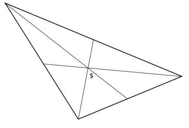
Figure 9: Triangle centroid (source: https://www.spatialanalysisonline.com/HTML/index.html)

For general polygons, using the same notation as before, the formulas required for the \(x\)- and \(y\)-components are (\(y\geq 0\)):

\(M2_{x}=\sum\limits_{i=1}^{n-1}\frac{(x_{i+1}y_{i}-x_{i}y_{i+1})(x_{i}+x_{i+1})}{6A}\qquad\qquad (17)\),

\(M2_{y}=\sum\limits_{i=1}^{n-1}\frac{(x_{i+1}y_{i}-x_{i}y_{i+1})(y_{i}+y_{i+1})}{6A}\qquad\qquad (18)\).

The formula arises as the weighted average of the centroids of triangles in a standard triangularization of the polygon, where the weights correspond to the triangle areas.

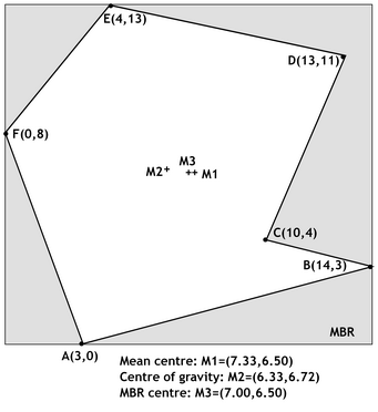
Figure 10: Polygon centroid M2 and alternative polygon centres (source: https://www.spatialanalysisonline.com/HTML/index.html)

Figure 10 shows a sample polygon with 6 nodes or vertices, \(A-F\), together with the computed locations of the mean center (\(M1\)), centroid (\(M2\)) as defined by the center of gravity, and the center (\(M3\)), of the Minimum Bounding Rectangle (or \(MBR\)) which is shown in gray.

Each of these three points fall within the polygon boundary in this example, and are fairly closely spaced. The \(MBR\) center is clearly the fastest to compute, but is not invariant under rotation and is the most subject to outliers — e.g. a single vertex location that is very different from the majority of the elements being considered. For example, if point \(B\) had (valid or invalid) coordinates of \(B(34,3)\) then we would find \(M1=(10.67,6.5)\), \(M2=(9.27,5.57)\) and \(M3=(17,6.5)\). \(M3\) is now well outside of the polygon, \(M1\) is close to the polygon boundary and \(M2\) remains firmly inside. None of these points minimizes the sum of distances to polygon vertices.

Despite the apparent robustness and widespread use of \(M2\), with a polygon of complex shape the centroid may well lie outside of its boundary. In the example illustrated in Figure 11 we have generated centroids for a set of polygons using the X‑Tools add-in for ArcGIS, and these produce slightly different results from those created by ArcGIS itself. ArcGIS includes a function, Features to Points, which will create polygon centers that are guaranteed to lie inside the polygon if the option INSIDE is included in the command. Manifold includes a Centroids|Inner command which performs a similar function.

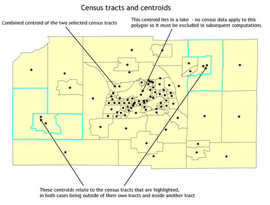
Figure 11: Center and centroid positioning (source: https://www.spatialanalysisonline.com/HTML/index.html)

An alternative to using the MBR is to find the smallest circle that completely encloses the polygon, taking the center of the circle as the polygon center (Figure 12, \(M4\)). This is the default in the Manifold GIS (viewable simply by selecting the menu option to View|Structure|Centroids) and/or using the Transform function “Centroids”. This procedure suffers similar problems to that of using the MBR. Yet another alternative is to find the largest inscribed circle, and take its center as the polygon center (Figure 121, \(M5\)). This approach has the advantage that the center will definitely be located inside the polygon, although possibly in an odd location, depending on the polygon shape. If the polygon is a triangle then M5 and M2 will coincide. Manifold supports location of centers of types \(M2, M3\) and \(M4\).

As we can also see in Figure 11 multiple polygons may be selected and assigned combined centers. In this example the combined center appears to have been computed from the MBR of the two selected census tracts, but different packages and toolsets may provide alternative procedures and thus positions. In such cases the center may be nowhere near any of the selected features, and if it is important to avoid such a circumstance the GIS may facilitate selection of the most central feature (e.g. the most central point or polygon) if one exists. In some instances the combined center calculation may be weighted by the value of an attribute associated with each polygon. This procedure will result in a weighted center whose location will be pulled towards regions with larger weights. However, in such cases the distribution of polygons used in the calculation may produce unrepresentative results.

This is apparent again in Figure 11 where a polygon center calculation for all census tracts in the western half of the region, weighted by farm revenues, would be pulled strongly to the east of the sub-region where many small urban tracts are found, even though these may have relatively low weights associated with them.

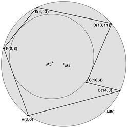
Figure 12: Polygon center selection (source: https://www.spatialanalysisonline.com/HTML/index.html)

11.4.2 Point sets

If \((x_i,y_i)\) are the coordinate pairs of a point set then the Mean Center, \(M1(x_0,y_0)\), is simply the average of the coordinate values, as we saw earlier:

\(M1(x_0,y_0)=\left(\frac{\sum\limits_i w_i x_i}{\sum\limits_i w_i},\frac{\sum\limits_i w_i y_i}{\sum\limits_i w_i}\right)\)

In this version of the expression for M1 there is an additional (optional) component, \(w_i\), representing weights associated with the points included in the calculation. For points sets the weights might be the number of crimes recorded at a particular location, or the number of beds in a hospital; for multiple polygons, where these are represented by their individual centers or centroids, the weights would typically be an attribute value associated with each polygon. Clearly if all weights=1 the formula simplifies to a calculation that is purely based on the coordinate values, with the number of points, \(n=∑w_i\).

M1 in this case is the center of gravity, or centroid, of the point set assuming the locations used in the calculation are treated as point masses. M1 is the location that minimizes the sum of (weighted) squared distance to all the points in the set, is simple and fast to compute, and is widely used. However, it is not the point that minimizes the sum of the (weighted) distance to each of the points. The latter is known sometimes as the (bivariate) “median center” (although Crimestat, for example, uses the term median center to be simply the middle values of the \(x\)- and \(y\)-coordinates). It is best described as the MAT point (the center of Minimum Aggregate Travel, \(M6\)). This point may be determined using the following iterative procedure, with \(M1\) as the initial pair \((x_0,y_0)\) and \(k=0,1,\dots\):