8 Data sources for GIS II - Global Navigation Satellite Systems and Coordinate Surveying
8.1 Introduction
Broadly defined, there are two general ways we measure the locations of geographic features. The first uses field measurements, and is described in this chapter. We travel to a feature and physically occupy a location to measure unknown X, Y, and often Z coordinates. Positioning and measurement systems have become quite sophisticated, incorporating satellite and laser technologies, primarily Global Navigation Satellite Systems (GNSS), as well as traditional ground surveying methods. Field measurements may be accurate to within millimeters (tenths of inches).
The second set of location measurement techniques uses remote data collection, primarily from aerial and satellite images. Coordinate positions may be obtained to within a few centimeters (inches) from properly collected, carefully processed images. GNSS are satellite-based technologies that give precise positional information, day or night, in most weather and terrain conditions (Figure 1). GNSS technologies may help navigate and track moving objects large enough to carry a receiver. Receivers shrink in size, weight, and power requirements each year.
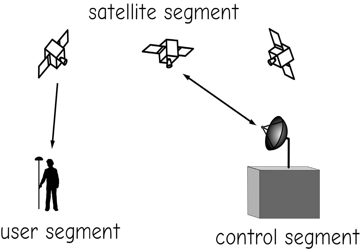
Figure 1: Segments of GNSS. (source: Bolstad, 2016)
Coordinate surveying encompasses traditional surveying through angle and distance measurements. Coordinate surveying is often combined with precise GNSS measurements. Because both measurement methods are important, they will be covered in this chapter, first by describing GNSS and coordinate surveying tools and methods, and then discussing common applications.
8.2 GNSS Basics
Because they are inexpensive, accurate, and easy to use, GNSS have significantly changed surveying, navigation, shipping, and other fields, and are also having a pervasive impact in the geographic information sciences. GNSS have become the most common method for field data collection in GIS.
As of 2015 there are two functioning GNSS systems and three more in various stages of development. The NAVSTAR Global Positioning System (GPS) was the first deployed and is the most widely used system. There is an operational Russian system named GLONASS that is increasingly used internationally; at the time of this writing there are 24 operational satellites and several spares in orbit, giving complete, 24-hour coverage worldwide. A third system, Galileo, is being developed by a consortium of European governments and industries, with a planned total of 30 satellites in the constellation, scheduled for completion in 2018. A fourth system, the Chinese Compass Satellite Navigation System, is also under development. A full constellation of 30 positioning satellites is planned, with global coverage. There is a regional system by the Indian government (IRNSS), with seven satellites giving coverage to south-central Asia, operational in 2015. Regional systems for India and Japan are also under development.
Note that GPS usually refers to the U.S. NAVSTAR system, but is widely used as a generic term for GNSS because it was the first broadly used satellite navigation system. In the following discussion we use GNSS as a generic term for all four systems, and use GPS to refer specifically to the U.S. NAVSTAR system.
There are three main components, or segments, of any GNSS (Figure 1). The first is the satellite segment. This is a constellation of satellites orbiting the Earth and transmitting positioning signals (Figure 2). The second component of any GNSS is a control segment. This consists of the tracking, communications, data gathering, integration, analysis, and control facilities. The third part of GNSS is the user segment, the GNSS receivers.
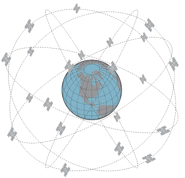
Figure 2: Satellite orbit characteristics for the NAVSTAR GPS constellation. (source: https://www.e-education.psu.edu/geog862/print/book/export/html/1768)
A receiver is an electronic device that records data transmitted by each satellite, and then processes these data to obtain threedimensional coordinates (Figure 3). There is a wide array of receivers and methods for determining position. Receivers are most often small, handheld devices with screens and keyboards, or electronic components mounted on trucks, planes, cargo containers, or cell phones.
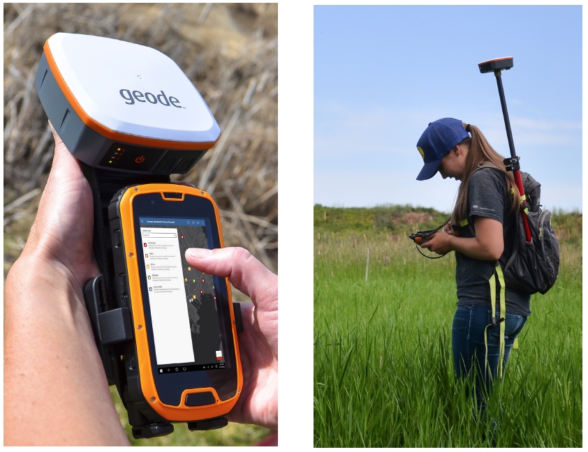
Figure 3: A hand-held GNSS receiver (left) and a GNSS receiver in use (right). (source: Bolstad, 2016)
The satellite and control segments differ for each GNSS. The NAVSTAR GPS includes a constellation of satellites orbiting the Earth at an altitude of approximately 20,000 km. Initial system design included 21 active GPS satellites and three spares, distributed among six offset orbital planes. Every satellite orbits the Earth twice daily, and each satellite is usually above the flat horizon for eight or more hours each day. Experimental and successive operational satellites have outlasted their design life, so there have typically been more than 24 satellites in orbit simultaneously. Between four to eight active satellites are typically visible from any unobstructed viewing location on Earth.
GPS is controlled by a set of ground stations. These are used to observe, maintain, and manage satellites, communications, and related systems. There are five tracking stations in the GPS system, with a Master Control Station in Colorado, United States, and the remaining stations spread across the planet. Data are gathered from a number of sources by the stations, including satellite health and status from each GPS satellite, tracking information from each tracking station, timing data from the U.S. Naval Observatory, and surface data from the U.S. Defense Mapping Agency. The Master Control Station synthesizes this information and broadcasts navigation, timing, and other data to each satellite. The Master Control Station also signals each satellite as appropriate for course corrections, changes in operation, or other maintenance.
The GLONASS system is another currently operating GNSS. GLONASS was initiated by the former Soviet Union in the early 1970s. Satellites were first launched in the early 1980s, and the system became functional in the mid-1990s. The GLONASS system was designed for military navigation, targeting, and tracking, and is operated by the Russian Ministry of Defense, with control and tracking stations similar to those for the NAVSTAR GPS system.
GLONASS was designed to include 21 active satellites and three spares. New designs have been phased in as older satellites have expired, and system managers have focused on maximizing coverage over Russia. The GLONASS system is stable enough, with a published renovation and maintenance plan, such that commercial manufacturers have developed dual GPS/GLONASS capable receivers.
Galileo also implements satellite, control, and user segments. There are 30 satellites planned for the complete Galileo constellation. Satellites are arranged in three orbital paths at a 54o orbital inclination, with a satellite altitude near 23,600 km above the Earth. This satellite constellation will provide better coverage of high northern latitudes than the U.S. NAVSTAR GPS system, to better serve northern Europe. Galileo will be managed through two control centers in Europe and 20 Galileo Sensor Stations spread throughout the world to monitor, communicate with, and relay information among satellites and the control centers.
8.2.1 GNSS Broadcast Signals
GNSS positioning is based on radio signals broadcast by each satellite. The NAVSTAR GPS satellites broadcast at a fundamental frequency of 10.23 MHz (MHz = Megahertz, or millions of cycles per second). GPS satellites also broadcast at other frequencies that are integer multiples or divisors of the fundamental frequency (Table 1). There are two carrier signals, L1 at 1575.42 MHz and L2 at 1227.6 MHz. These carrier signals are modulated to produce two coded signals, the C/A code at 1.023 MHz and the P code at 10.23 MHz. The L1 signal carries both the C/A and P codes, while the L2 carries only the P code. Planned upgrades to the GPS system include additional, higher-power L bands that may provide additional information and be easier to receive. These other signals have been added to improve function, for example, the L2C to ease GPS tracking for navigation, L5 for worldwide safety of life applications, and M for enhanced military applications. The coded signals (C/A, P, and M) are sometimes referred to as the pseudorandom code, because they appear quite similar to random noise. However, short segments of the code are unique for each satellite and time. A receiver decodes each signal to identify the satellite, transmission time, and satellite position at the time the signal was sent. The receiver combines this information from multiple satellites for positioning. The coded signal does repeat, but the repeat interval is long enough to not cause problems in positioning.
Table 1: GPS Signals
| Name | Frequency (MHz) |
|---|---|
| L1, L1C | 1575.42 |
| L2, L2CM, L2CL | 1227.6 |
| L5 | 1176.45 |
| P, M | 10.23 |
| C/A | 1.023 |
(source: Bolstad, 2016)
Positions based on carrier signal measurements (L1, L2, and L5 frequencies for the NAVSTAR GPS, and sometimes referred to as carrier phase measurements) are inherently more accurate than those based on the code signal measurements. The mathematics and physics of carrier measurement are better suited for making positional measurements. However, the added accuracy incurs a cost. Carrier measurements require more sophisticated and expensive receivers. Perhaps a greater constraint on carrier measurements is that carrier receivers must record signals for longer periods of time than C/A code receivers. If the satellite passes behind n obstruction, such as a building, mountain, or tree, the signal may be momentarily lost and carrier phase measurements begun anew. Satellite signals are frequently lost in heavily obstructed environments, substantially reducing the efficiency of carrier phase data collection. These constraints have decreased with modern receivers, often tracking multiple GNSS systems with hundreds of channels, but there are still more exacting requirements for carrier phase positioning.
Each GPS satellite also broadcasts data on satellite status and location. Information includes an almanac, data used to determine the status of satellites in the GPS constellation. The broadcast also includes ephemeris data for the satellite constellation. These ephemerides allow a GPS receiver to accurately calculate the position of the broadcasting satellite and the expected positions of other satellites. Satellite health, clock corrections, and other data are also transmitted.
The other GNSS systems operate in a similar manner, with base, or carrier frequencies, and modulated or coded signals embedded within these carriers (Figure 4). GLONASS, the only other fully operational GNSS in 2011, broadcasts L1 and L2 carriers similar to GPS, and an additional L1/L10 and experimental G3 signal at higher and lower frequencies. Galileo plans include the broadcasts of a range of signals on several fundamental carriers, including one that overlaps with the GPS and GLONASS L1 signals at approximately 1575 MHz, with several coded signals planned at lower frequencies.
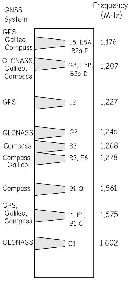
Figure 4: Existing and proposed GNSS broadcast signals, frequencies, and positioning services. Signals are spaced to avoid interference, or coded where they overlap. Frequencies are not spaced to scale (courtesy ESA). (source: Bolstad, 2016)
Substantial effort has been directed at ensuring the NAVSTAR, GLONASS, and Galileo systems do not interfere with each other, and are as compatible as practical. All three systems will broadcast in the 1575 MHz range, with signals coded differently to avoid interference. This simplifies the production of dual-system receivers that are capable of using multiple GNSS signals, improving coverage, accuracy, and efficiency, particularly under difficult data collection conditions. When all GNSS constellations are fully operational, there may be as many as 70 satellites broadcasting in this range, greatly improving coverage.
There is a notable overlap in some frequencies used by the Galileo and Chinesebased Compass system. While there is the possibility for mutual interference in signals, it is likely that the Compass and Galileo systems will be operated to avoid this.
8.2.2 Range Distances
GNSS positioning is based primarily on range distances determined from the carrier and coded signals. A range distance, or range, is a distance between two objects. For GNSS, the range is the distance between a satellite in space and a receiver (Figure 5). GNSS signals travel approximately at the speed of light. The range distance from the receiver to each satellite is calculated based on signal travel time from the satellite to the receiver:
\(Range = speed\ of\ light\ *\ travel\ time.\) (8.1)
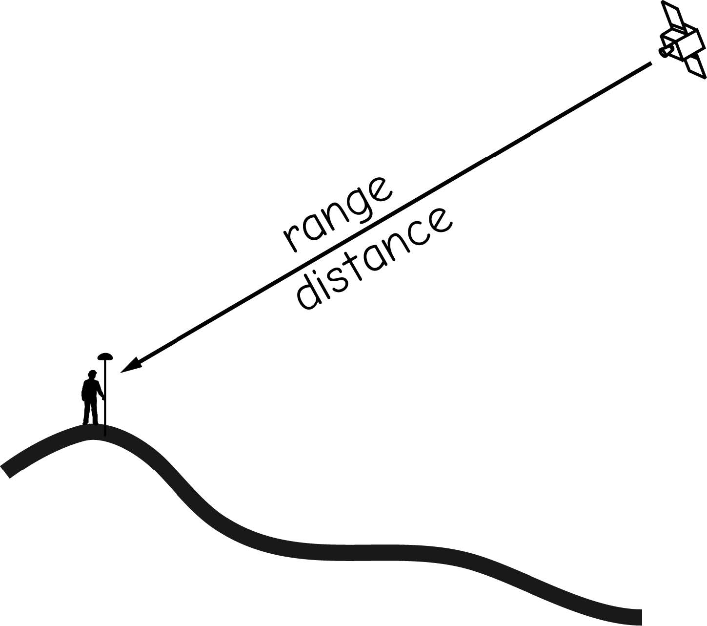
Figure 5: A single satellite range measurement. (source: Bolstad, 2016)
Coded signals are used to calculate signal travel time by matching sections of the code. Timing information is sent with the coded signal, allowing the GNSS receiver to calculate the precise transmission time for each code fragment. The GNSS receiver also observes the reception time for each code fragment. The difference between transmission and reception times is the travel time, which is then used to calculate a range distance (Figure 6). Range measurements can be repeated quite rapidly, typically up to a rate of one per second; therefore several range measurements may be made for each satellite in a short period of time.
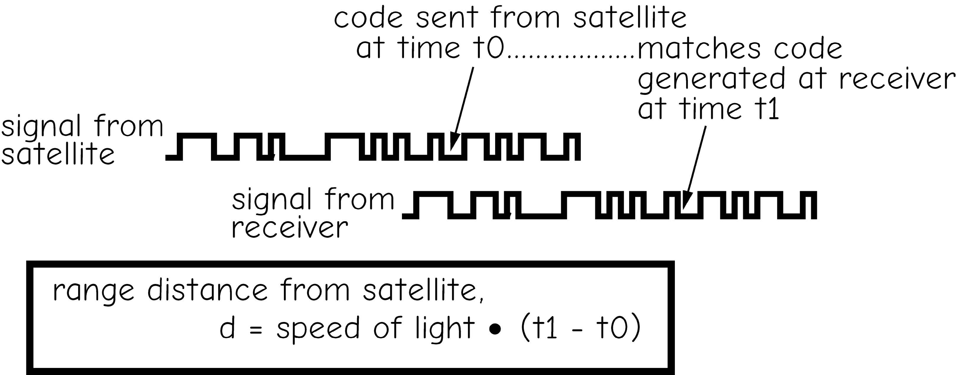
Figure 6: A decoded C/A satellite signal provides a range measurement. (source: Bolstad, 2016)
Carrier phase GNSS is also based on a set of range measurements. In contrast to coded signals, the phase of the satellite signal is measured. Each individual wave transmitted at a given frequency is identical, and at any given point in time there is some unknown integer number of waves plus a partial wave that fit in the distance between the satellite and the receiver. Carrier signal observations over extended intervals allow the calculation of wavelength number over the measurement interval, and then the calculation of very precise satellite ranges.
Simultaneous range measurements from multiple satellites are used to estimate a receiver’s location. A range measurement is combined with information on satellite location to define a sphere. A range measurement from a single satellite restricts the receiver to a location somewhere on the surface of a sphere centered on the satellite (Figure 7a). Range measurements from two satellites identify two spheres, and the receiver is located on the circle defined by the intersection of the two spheres (Figure 7b). Range measurements from three satellites define three spheres, and these three spheres will intersect at two points (Figure 7c). A sequence of range measurements through time from three satellites will reveal that one of the points remains nearly stationary, while the other point moves rapidly through space. The point moves through space because the size and relative geometry of the spheres change through time as the satellites change positions. If system and receiver clocks were completely accurate, it would be possible to determine the position of a stationary receiver by taking measurements from three satellites over a short time interval. However, simultaneous measurements from four satellites (Figure 7d) are usually required to reduce receiver clock errors and to allow instantaneous position measurement with a moving receiver, for example, on a plane, in a car, or while walking. Data may be collected from more than four satellites at a time, and this usually improves the accuracy of position measurements.
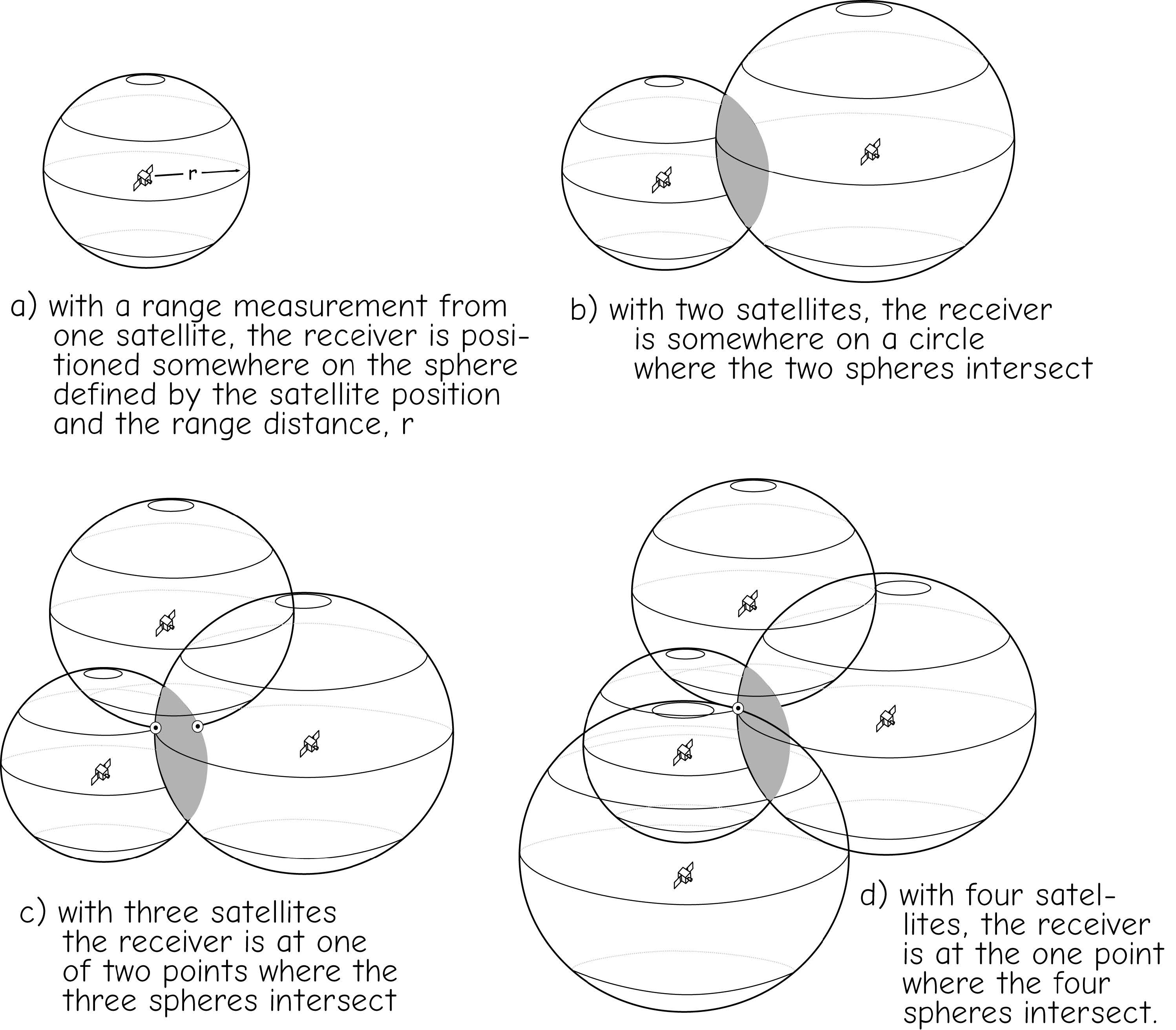
Figure 7: Range measurements from multiple GNSS satellites. Range measurements are combined to narrow down the position of a GNSS receiver. Range measurements from more than four satellites may be used to improve the accuracy of a measured position. (adapted from Hurn, 1989).(source: Bolstad, 2016)
8.2.3 Positional Uncertainty
Errors in range measurements and uncertainties in satellite location introduce errors into GNSS-determined positions. Range errors vary substantially even if range measurements are taken just a few seconds apart. Errors in the ephemeris data lead to erroneous estimates of the satellite position, causing location error. The intersection of the range spheres changes through time, even when the GNSS receiver is in a fixed location. This results in a band of range uncertainty encompassing the GNSS receiver position (Figure 8).
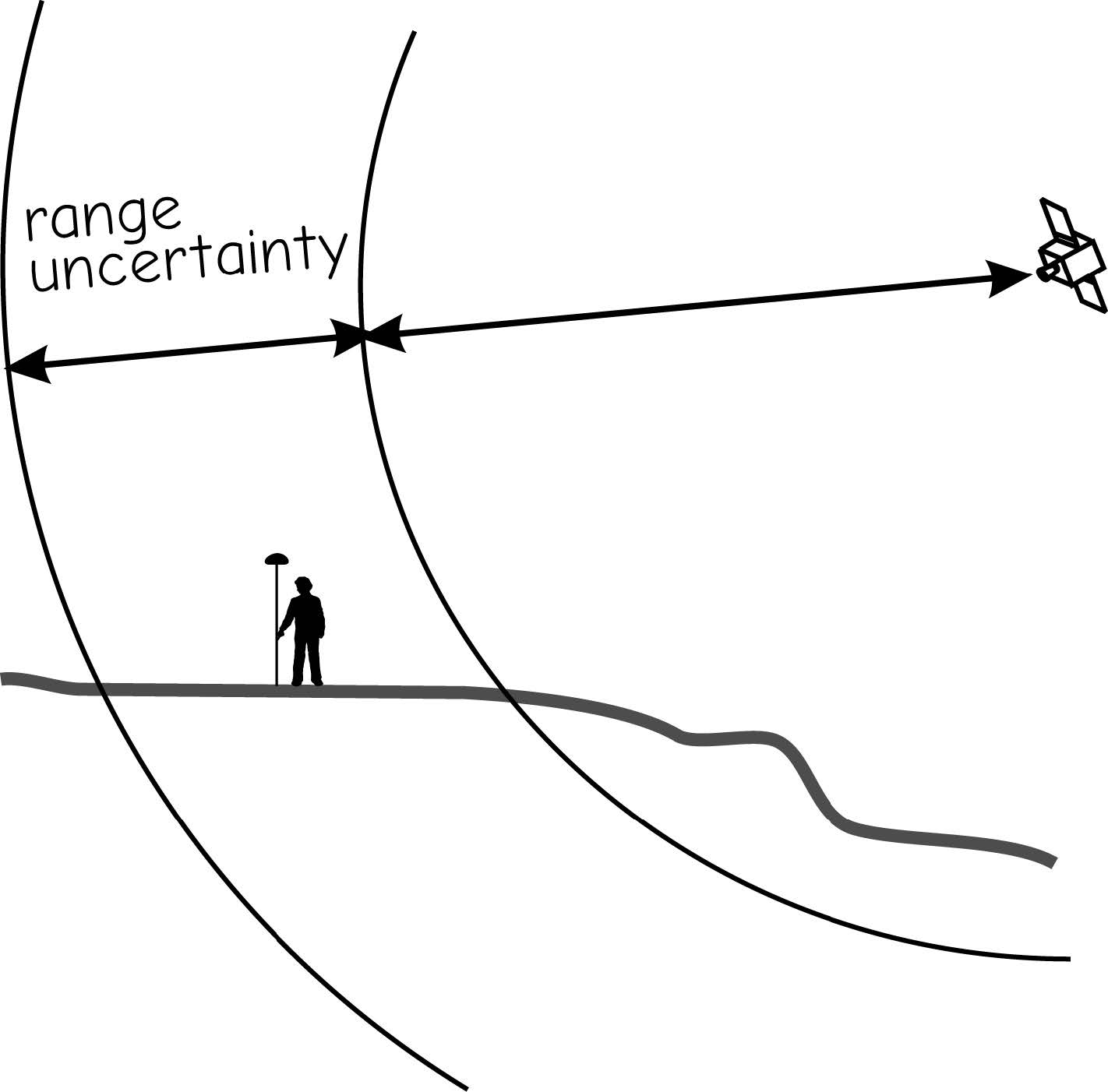
Figure 8: Uncertainty in range measurements leads to positional errors in GNSS measurements.(source: Bolstad, 2016)
Several methods are used to improve our estimates of receiver position. One common method involves collecting multiple estimates of stationary receiver location. Most receivers may estimate a new position, or fix, every second. Receivers collect and average multiple position fixes, yielding a mean position estimate. Multiple fixes enable the receivers to estimate the variability in the position locations, for example, a standard deviation, predicted accuracy, or some other figure of merit. While the standard deviation provides no information on the absolute error, it does allow some estimate of the precision of the mean GNSS position fix. The magnitude and properties of this variation may be useful in evaluating GNSS measurements and the source of errors. However, multiple position fixes are not possible when data collection takes place while moving, for example, when determining the location of an airborne plane. Also, averaging does not remove any bias in the calculated position. Alternative methods for reducing positional error rely on reducing the several sources of range errors.
8.2.4 Sources of Range Error
Ionospheric and atmospheric delays aremajor sources of GNSS positional error. Range calculations incorporate the speed of light. Although we usually assume the speed of light is constant, this is not true. The speed of light is constant only while passing through a uniform electromagnetic field and in a vacuum. The Earth is surrounded by a blanket of charged particles called the ionosphere. These charged particles are formed by incoming solar radiation, which strips electrons from elements in the upper atmosphere. Changes in the charged particle density through space and time result in a changing electromagnetic field surrounding the Earth.
The atmosphere is below the ionosphere, and atmospheric density is significantly different from that of a vacuum. Variation in atmospheric density is due largely to changes in temperature, atmospheric pressure, and water vapor. Range errors occur because the GNSS signal velocity is altered slightly as it passes through the ionosphere and atmosphere; some systems allow satellite screening based on horizon angle, to improve accuracy (Figure 9).
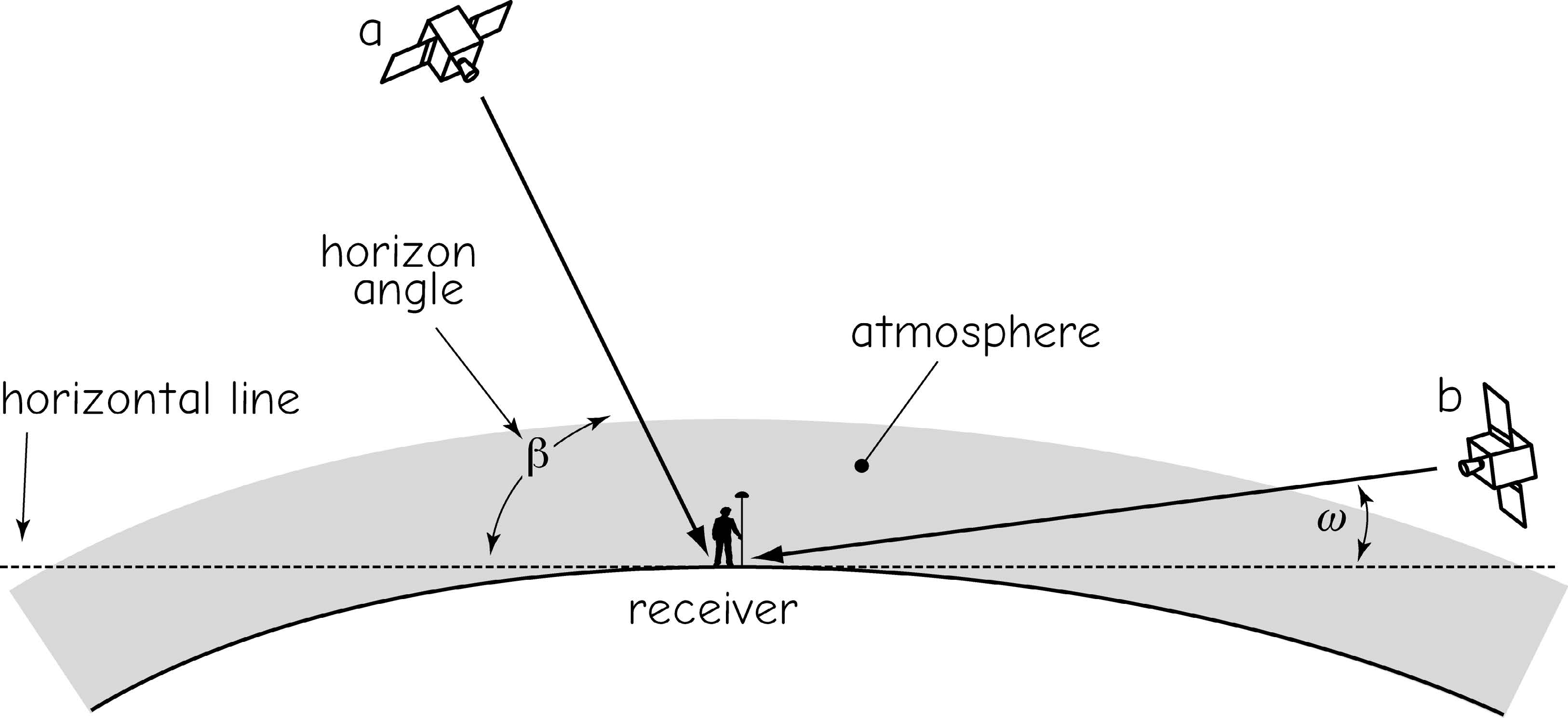
Figure 9: GNSS receivers often discard signals from satellites near the horizon. As this image shows, signals from satellites high above the horizon (a) with high horizon angles (\(\beta\)) have shorter path lengths in the atmosphere than low-angle satellites (b, with angle \(\omega\)). Atmospheric delays and hence range errors are larger for satellites with low horizon angles. Typically a “mask” is set at approximately 15 degrees above the horizon, and satellites are ignored if they are below this limit.(source: Bolstad, 2016)
We may reduce ionospheric errors by adjusting the value used for the speed of light when calculating the range distance. Physical models can be developed that incorporate measurements of the ionospheric charge density. Because the charge density varies both around the globe and through time, and because there is no practical way to measure and disseminate the variation in charge density in a timely manner, physical models are based on the average charge.
These physical models reduce the range error somewhat. Alternatively, correction could be based on the observation that the change in the speed of light depends on the frequency of the light. Specialized dual-frequency receivers collect information on multiple GNSS signals simultaneously, and use sophisticated physical models to remove most of the ionospheric errors. Dual-frequency receivers find more limited use, in part because they more expensive than codebased receivers, and because they must maintain a continuous fix for a longer period of time. Finally, there are no good models for atmospheric effects, thus there is no analytical method to remove range errors due to atmospheric delays.
System operation and delays are other sources of range uncertainty. Small errors in satellite tracking cause errors in satellite positional measurements. Timing and other signals are relayed from globally distributed monitoring stations to the Master Control Center and up to the satellites, but there are uncertainties and delays in signal transmission, so timing signals may be slightly offset. Atomic clocks on the satellite may be un-synchronized or in error, although this is typically one of the smaller contributions to positional errors.
Receivers also introduce errors into GNSS positions. Receiver clocks may contain biases or may use algorithms that do not precisely calculate position. Signals may reflect off of objects prior to reaching the antenna. These reflected, multipath signals travel a farther distance than direct GNSS signals and so introduce an offset into GNSS positions. Multipath signals often have lower power than direct signals, so some multipath signals may be screened by setting a threshold signal-to-noise ratio. Signals with high noise relative to the mean signal strength are ignored. Multipath signals may also be screened by properly designed antennas. Multipath signals are most commonly a problem in urban settings that have an abundance of corner reflectors, such as the sides of buildings and streets.
8.2.5 Satellite Geometry and Dilution of Precision
The geometry of the GNSS satellite constellation is another factor that affects positional error. Range errors create an area of uncertainty perpendicular to the transmission direction of the GNSS signal. These areas of uncertainty may be visualized as a set of nested spheres, with the true position somewhere within the volume defined by the intersection of these nested spheres (Figure 10). These areas of uncertainty from different satellites intersect, and the smaller the intersection area, the more accurate the position fixes are likely to be (Figure 11). Signals from widely spaced satellites are complementary because they result in a smaller area of uncertainty. Signals from satellites in close proximity overlap over broad areas, resulting in large areas of positional uncertainty. Widespread satellite constellations provide more accurate GNSS position measurements.
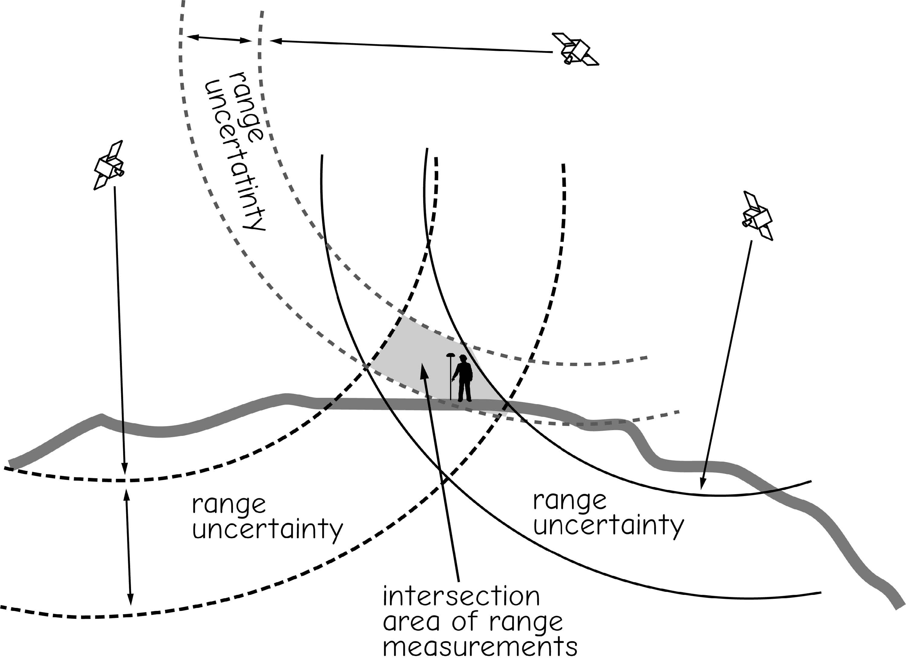
Figure 10: Relative GPS satellite position affects positional accuracy. Range uncertainties are associated with each range measurement. These combine to form an area of uncertainty at the intersection of the range measurements..(source: Bolstad, 2016)
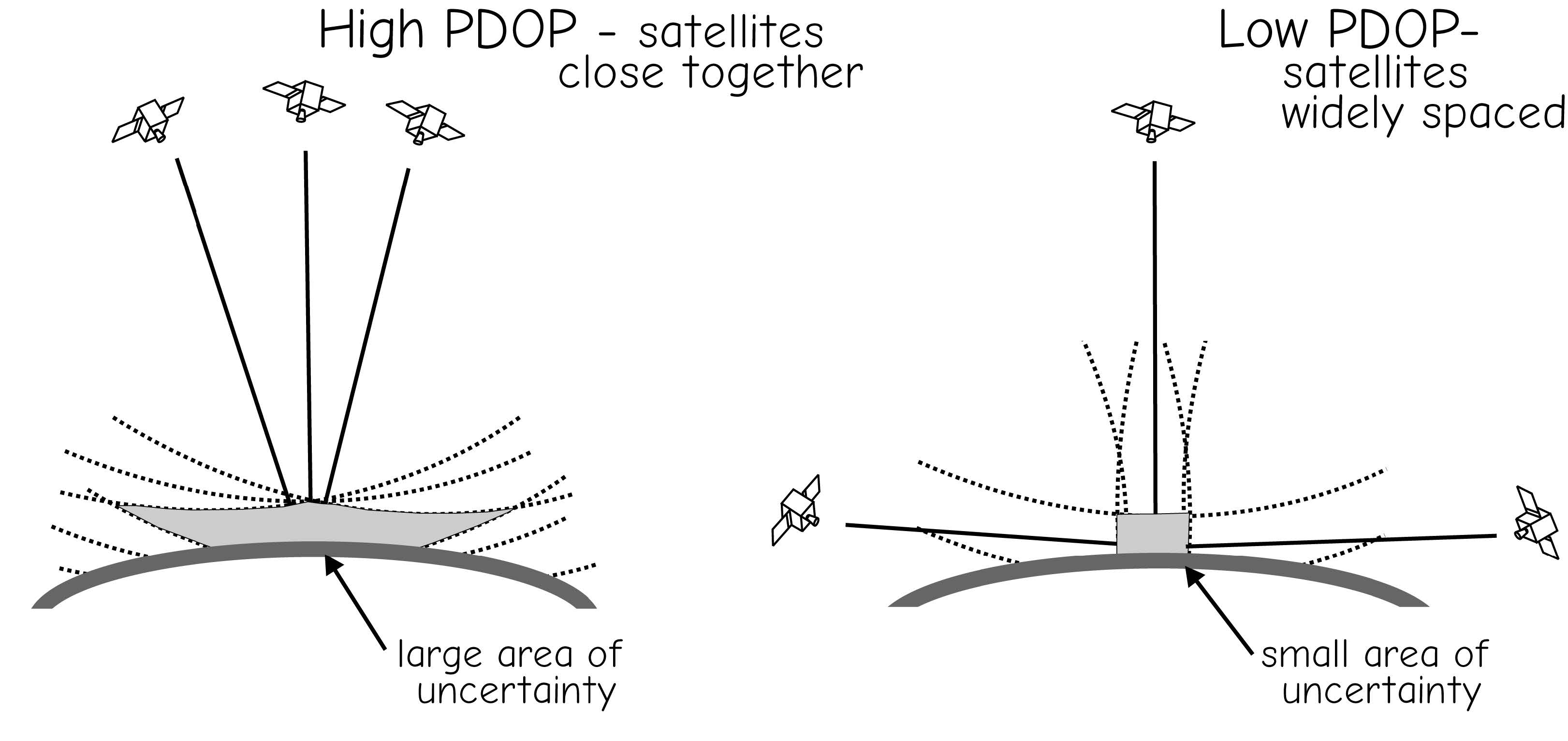
Figure 11: GPS satellite distribution affects positional accuracy. Closely spaced satellites result in larger positional errors than widely spaced satellites. Satellite geometry is summarized by PDOP with lower PDOPs indicating better satellite geometries..(source: Bolstad, 2016)
Satellite geometry is summarized in a number called the Dilution of Precision, or DOP. There are various kinds of DOPs, including the Horizontal (HDOP), Vertical (VDOP), and Positional (PDOP) Dilution of Precision. The PDOP is most used and is the ratio of the volume of a tetrahedron created by the four most widespread, observed satellites to the volume defined by the ideal tetrehedron. This ideal tetrahedron is formed by one satellite overhead and three satellites spaced at 120-degree intervals around the horizon. This constellation is assigned a PDOP of one, and closer groupings of satellites have higher PDOPs. Lower PDOPs are better. Most GNSS receivers review the almanac transmitted by the GNSS satellites and attempt to select the constellation with the lowest PDOP. If this best constellation is not available, for example, some satellites are not visible, successively poorer constellations are tested until the best available constellation is found. The receivers typically provide a measurement of PDOP while data are collected, and a maximum PDOP threshold may be specified. Data are not gathered when the PDOP is above the threshold value.
Range errors and DOPs combine to affect GNSS position accuracies. There are many sources of range error, and these combine to form an overall range uncertainty for the measurement from each visible GNSS satellite. If more precise coordinate locations are required, then the choices are to use equipment that makes more precise range measurements, and/or to collect data when DOPs are low.
GNSS accuracies depend on the type of receiver, atmospheric and ionospheric conditions, the number of range measurements, the satellite constellation, and the algorithms used for position determination (Figure 12). Observed GPS error distributions for various receivers under open sky conditions (a through c) and mean error under open sky and dense deciduous forest canopy (d). Results show highest accuracies for a professional grade GNSS receiver (panel a, TRIMBLE 6H, post-processed carrier phase differential correction, < 20 km to a base station) a professional grade GNSS receiver with WAAS real-time correction (b), and an inexpensive consumer-grade GNSS (c, Garmin etrex). Mean errors for both open sky and under forest canopy are shown in panel d for these three receivers/configurations, and for an iPhone 5 and a similar tablet GPS. Centimeter-level accuracies are available with the best equipment under optimal conditions, but less expensive receivers and obstructed skies reduce accuracies. In some instances the individual fix error is important, for example, when digitizing lines or polygon boundaries, while average errors may be more important when collecting point features, allowing multiple fixes. Note that errors decrease as technology improves, but the higher-priced receivers may not be more expensive over the life of a project if lower accuracies require significant manual editing for GNSS collected data.Current C/A code receivers typically provide accuracies between 3 and 30 m for a single fix. Errors larger than 100 m for a single fix occur occasionally. Accuracies may be improved substantially, to between 2 and 15 m, when multiple fixes are averaged. The longer the data collection time, the greater the accuracy. Improvements come largely from reducing the impact of rarer, large errors, but average accuracies are rarely below one m when using a single C/A code receiver.
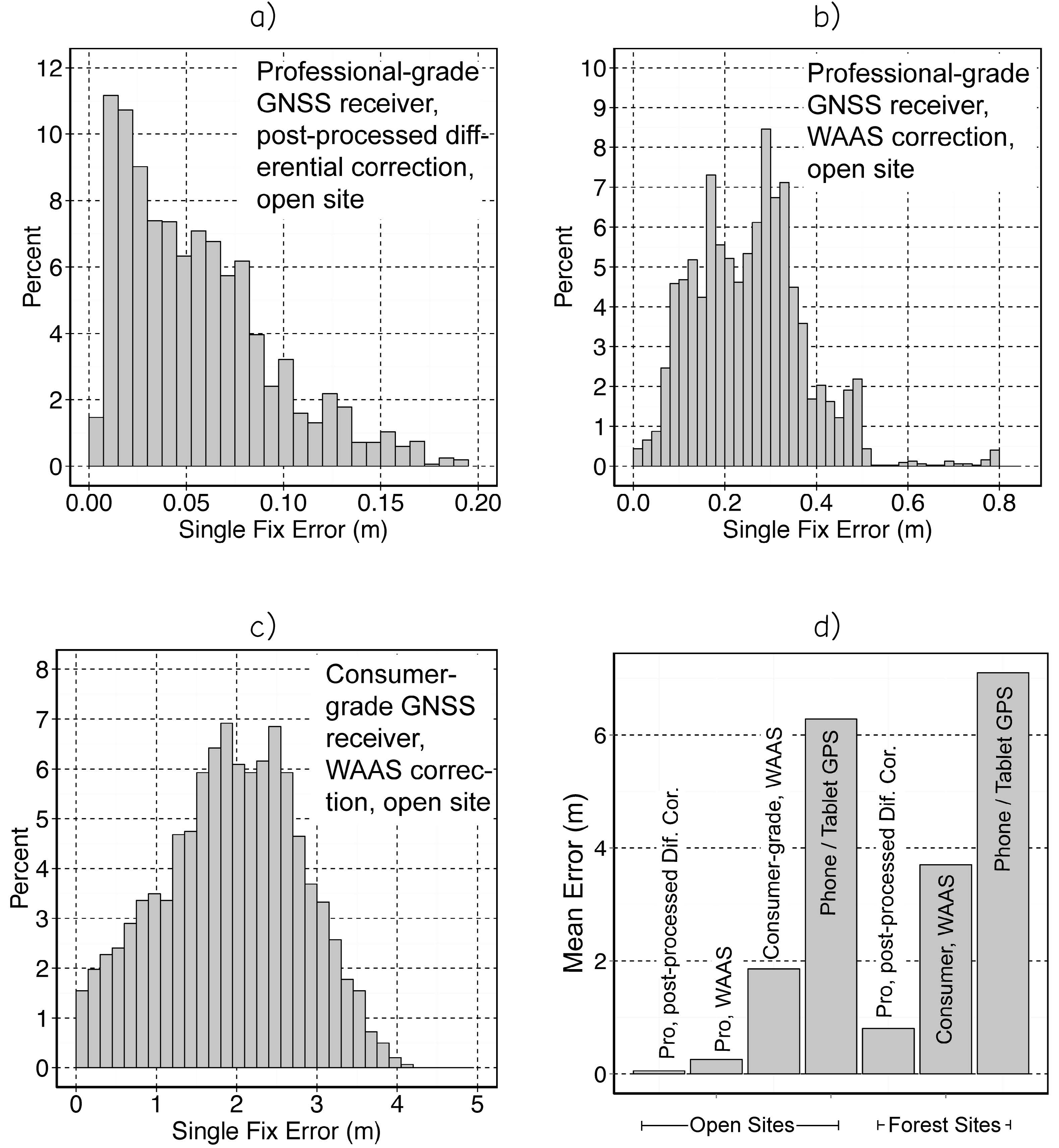
Figure 12: Observed GPS error distributions for various receivers under open sky conditions.(source: Bolstad, 2016)
Accuracies when using carrier phase or similar receivers are much higher, on the order of a few centimeters. These accuracies come at the cost of longer data collection times, and are most often obtained when using differential correction, a process described in the following section.
8.2.6 Differential Correction
The previous sections have focused on GNSS position measurements collected with a single receiver. This operating mode is known as autonomous GNSS positioning. An alternative method, known as differential positioning, employs two or more receivers. Differential positioning measurements are used primarily to remove most of the range errors and thus greatly improve the accuracy of GNSS positional measurements (Figure 12). However, differential positioning is not always employed, because single receiver positioning is accurate enough for some applications, and differential positioning requires more time and/or greater expense.
Differential GNSS positioning entails establishing a base station receiver at a known coordinate point (Figure 13). The true coordinate location of the base station is typically determined using high-accuracy surveying methods, for example, repeated astronomical observations, highest-accuracy GNSS, or precise ground surveys.
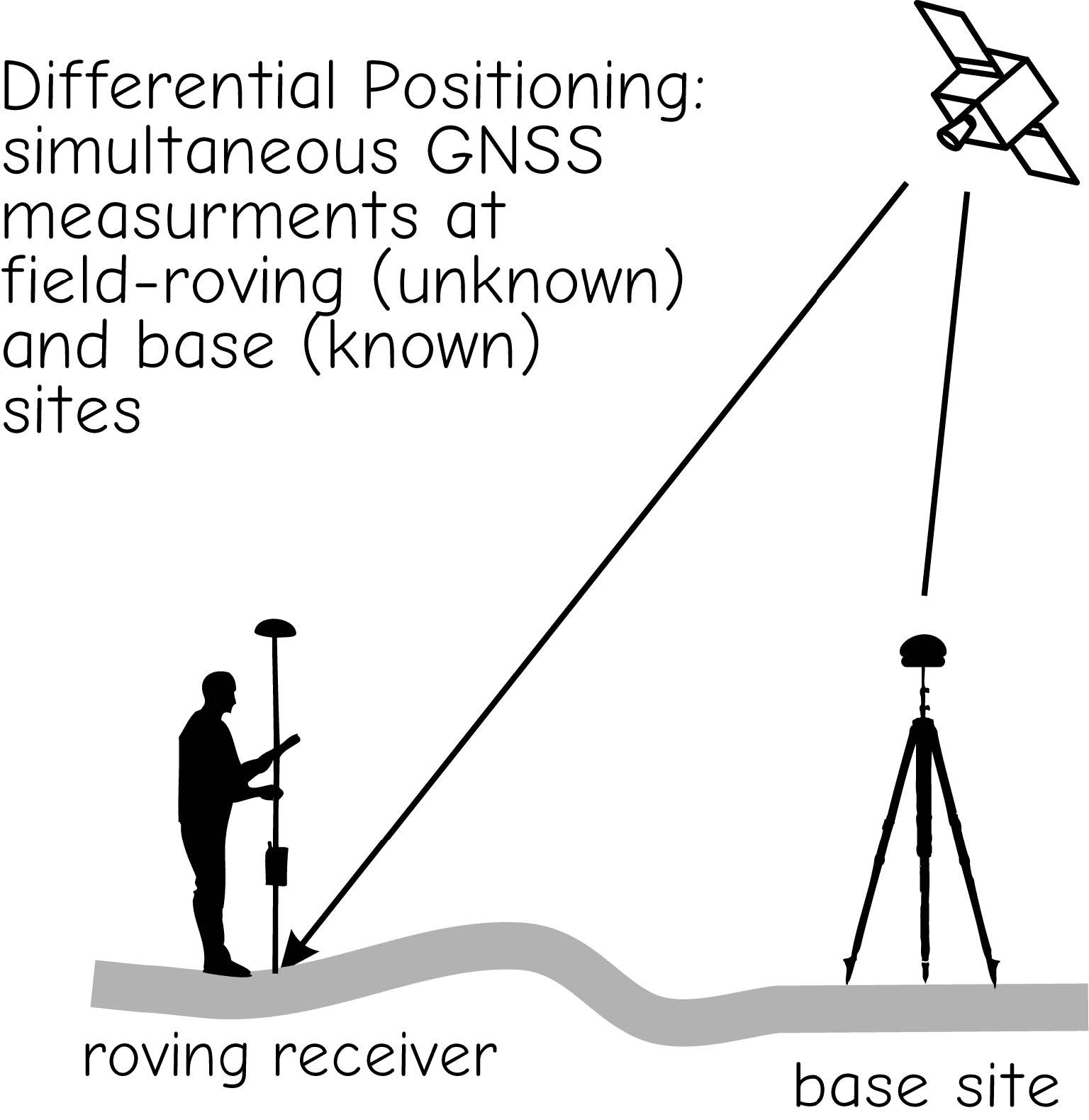
Figure 13: Differential GNSS positioning.(source: Bolstad, 2016)
We use the base station to estimate a portion of the range measurement errors for each position fix. Remember that GNSS is based on a set of range measurements, and these range measurements contain errors. Some of these errors are due to uncertainty in the measured travel times from the satellite to the receiver. These travel time errors, also known as timing errors, are often among the largest sources of positional uncertainty.
In differential correction we use the known base station position to estimate the timing errors and hence range errors. Each GNSS satellite broadcasts its position along with the ranging signal. The “true” distance from a given satellite to the base station can be calculated because the base station and satellite locations are known. However, note the qualifying quote marks around the “true.” We cannot exactly define where the satellite is, and the base station coordinates have some (usually small) level of uncertainty associated with them. However, if we are very careful about surveying the location of our base station, then the errors in the base-to-satellite measurement are almost always smaller than the range errors contained in our uncorrected timing measurement.
The difference between the true distance and GNSS-measured distance is used to estimate the timing error for a given satellite at any given second. The timing errors change each second, so they should be measured frequently.
Timing corrections may be applied to the range measurements collected by a roving receiver (Figure 5-15). These roving receivers are used to measure GNSS positions at field locations with unknown coordinates. The timing error, and hence range error, for each satellite observed at a field location is assumed to be the same as the range error observed simultaneously at the base station. We adjust the timing of each satellite measurement made by the rover, then calculate the rover’s position in the field. This adjustment usually reduces each range error and substantially improves each position fix taken with the roving field receivers.
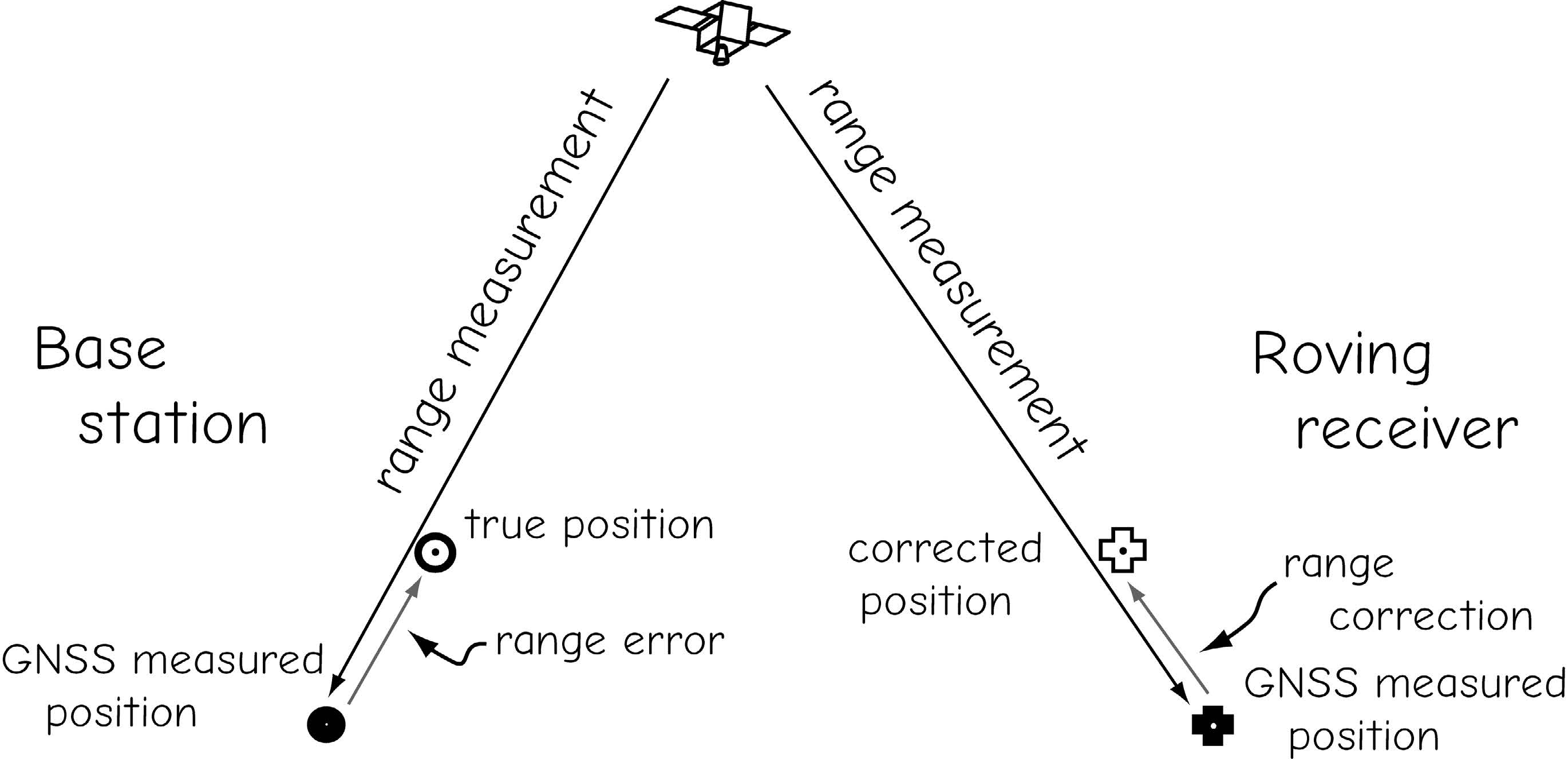
Figure 14: Differential correction is based on measuring GNSS timing and range errors at a base station, and applying these errors as corrections to simultaneously measured rover positions.(source: Bolstad, 2016)
The timing errors change across the surface of the Earth, and this places a restriction on the use of differential GNSS correction. Our roving receivers must be “near” our base station for differential correction to work. A substantial portion of the range error is due to atmospheric and ionospheric interference with the GNSS signal. Fortunately, these conditions often vary slowly with distance through the atmosphere, so interaction in one location is likely to be similar to interaction, and thus error, in a nearby location. Therefore, as long as the rover is close to the base station we may expect differential correction to improve our position measurements.
Differential correction requires the base station and roving receivers to collect data from a similar set of satellites. We cannot fix a timing error we do not measure. Any four satellites providing acceptable PDOPs will suffice.
The simultaneous viewing requirement limits the distance between the base and roving receivers. The farther apart the receivers, the more likely they will not view the same set of satellites. While differential positioning has been successful at distances of over 1500 km (1000 m), best performance is achieved when the roving receiver is within 300 km (180 mi) of the base station, and closer is usually better.
Successful differential correction also requires near simultaneity in the base and rover measurements. Errors change rapidly through time. If the base and rover measurements are collected more than a few tens of seconds apart, they do not correspond to the same set of errors, and thus the difference at the base station cannot be used to correct the rover data. Many systems allow data collection to be synchronized to a standard timing signal, thereby ensuring a good match when the error vectors are applied to correct the roving receiver GNSS data.
Base station data and roving receiver data must be combined for differential correction. A base station correction may be calculated for each fix, but this correction must somehow be joined with the roving receiver data to apply the correction. Many receivers allow large amounts of data to be stored, either internal to the receiver, or in an attached computer. Files may be downloaded from the base station and roving units to a common computer. Software provided by most GNSS system vendors is then used to combine the base and rover data and compute and apply the differential corrections to the position fixes. This is known as post processed differential correction, as corrections are applied after, or post, data collection (Figure 15, top).
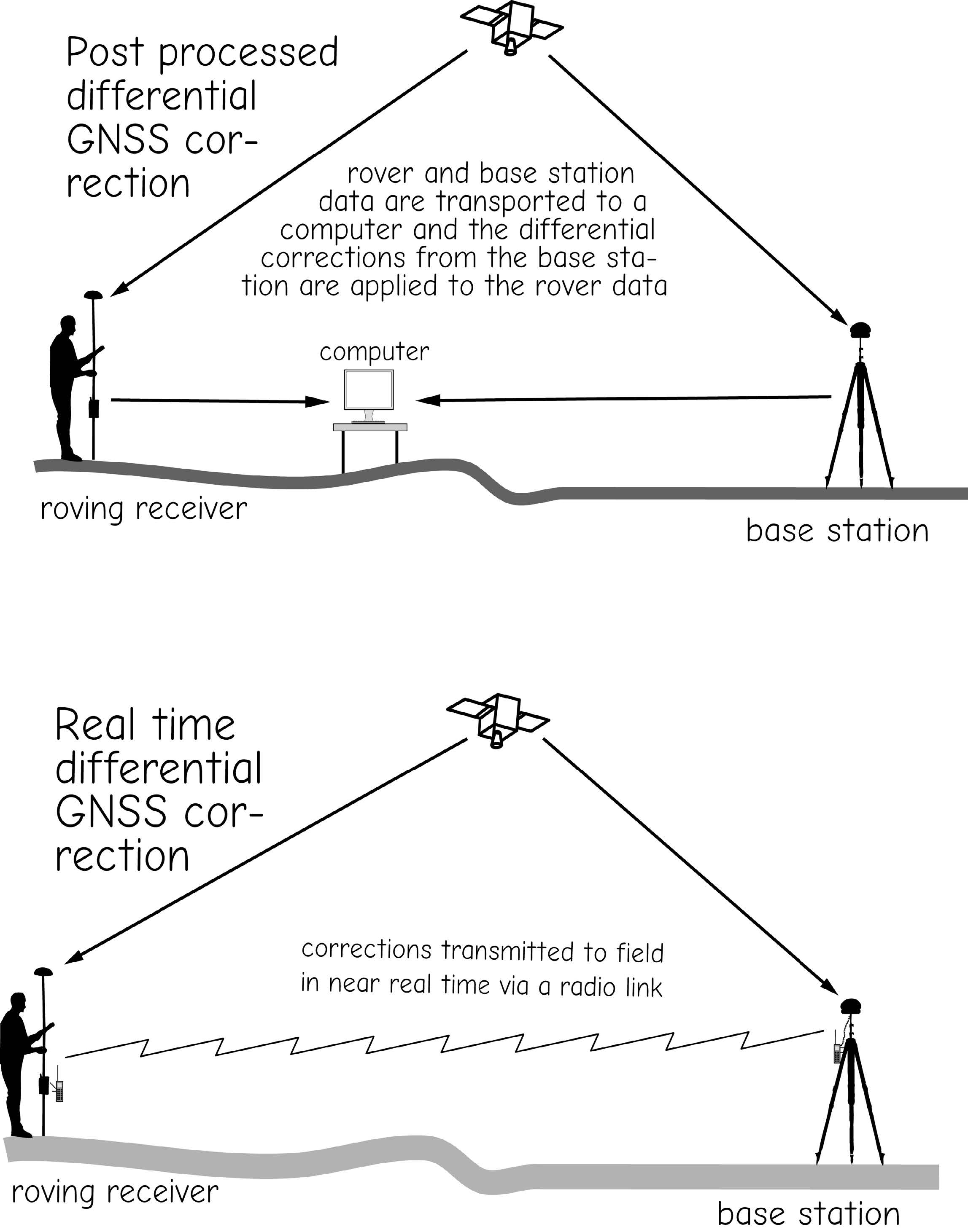
Figure 15: Post-processed and real time differential GNSS correction.(source: Bolstad, 2016)
8.2.7 Real Time Differential Positioning
An alternative GNSS correction method, known as real time differential correction, may be appropriate when precise navigation is required. Real time differential correction requires some extra equipment and there is some cost in slightly lower accuracy when compared to post-processed differential GNSS. However, the accuracy of real time differential correction is substantially better than autonomous GNSS, and accurate locations are determined while still in the field.
Real time differential GNSS positioning requires a communications link between the base station and the roving receiver (Figure 15, bottom). Typically the base station is connected to a radio transmitter and an antenna. FM radio links are often used due to their longer range and good transmission through vegetation, into canyons or deep valleys, or into other constrained terrain. The base station collects a GNSS signal and calculates range distances. The error is calculated for each range distance. The magnitude and direction of each error is passed to the radio transmitter, along with information on the timing and satellite constellation used. This continuous stream of corrections is broadcast via the base station radio and antenna.
Roving GNSS receivers are outfitted with a receiving radio, and any receiver within the broadcast range of the base station may receive the correction signal. The roving receiver is also recording GNSS data and calculating position fixes. Each position fix by the roving receiver is matched to the corresponding correction from the base station radio broadcast. The appropriate correction is then applied to each fix and accurate field locations are computed in real time. Real time differential correction requires a broadcasting base station; however, every user is not required to establish a base station and radio or other communication system.
The U.S. Coast Guard has established a set of GPS radio beacons in North America that broadcast a standardized correction signal (Figure 16). A compatible GPS receiver near these beacons can use the signal for differential correction. These GPS beacon receivers typically have an additional antenna and electronics for processing the beacon signal. Beacons were originally to aid in ship navigation in coastal and major inland waters, so beacons are concentrated near coastal and major inland waters. This system has become the Maritime Differential GPS systems and is part of a National Differential GPS system (NDGPS) under development with collaboration of Federal Departments of Transportation, Homeland Security, and others. This will support navigation and positioning in areas distant from the Coast Guard network. Many GPS manufacturers sell beacon receiver packages that support real-time correction using the beacon signal.
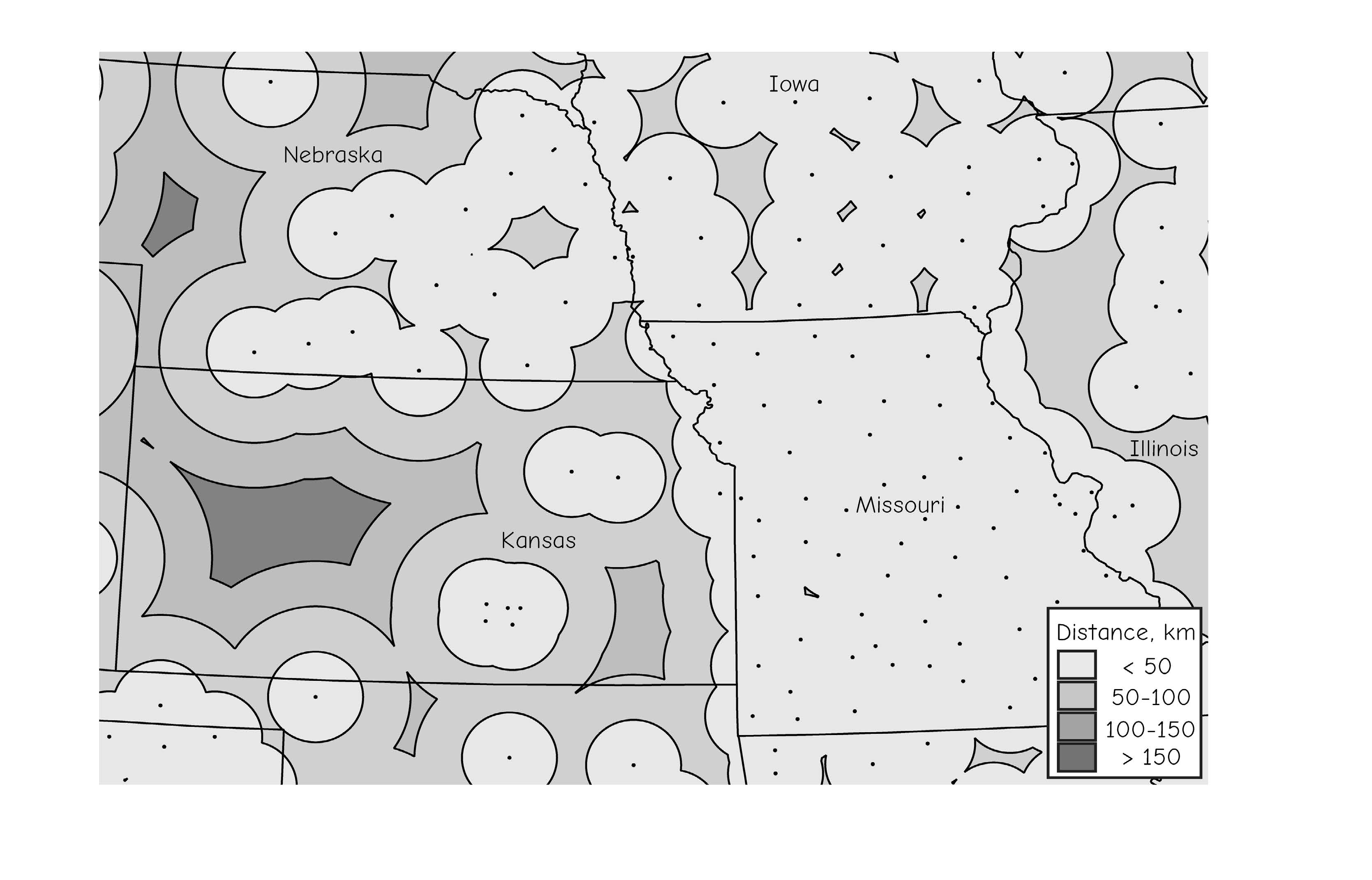
Figure 16: The location of RTK available stations (dots) in the central U.S, in April, 2015. Station locations and distances from the nearest beacon are shown.(source: Bolstad, 2016)
8.2.8 WAAS, Augmentation, and Satellite-based Corrections
There are alternatives to ground-based differential correction for improving the accuracy of GNSS observations. One alternative, known as the Wide Area Augmentation System (WAAS), is administered by the U.S. Federal Aviation Administration to provide accurate, dependable aircraft navigation.
WAAS uses a network of ground reference stations spread across North America to correct GPS signals. A generalized correction for each station is broadcast from geostationary satellites, and applied real time for improved accuracy in roving receivers. Tests indicate individual errors are less than 7 m 95% of the time, and average errors less than 3 m, an improvement over uncorrected C/A code (Figure 12). WAAS is often unavailable at extreme northern latitudes, where equatorial geostationary satellites are often not visible.
The Japanese government has taken a different approach, with three satellites in the QZSS system that augment the GPS constellation. Orbital paths keep at least one satellite high over Japan, improving PDOPS, satellite visibility, and communication in urban canyons, common in Japanese cities.
8.2.9 Real Time Kinematic and Virtual Reference Stations
The highest accuracy differential correction is provided with dual-frequency, carrier phase positioning, often called **real time kinematic (RTK) GNSS*. The amount of ionospheric delay is different for different frequencies, so by comparing signals, such as the GPS carriers L1 and L2, the ionospheric delays may be estimated and removed. The CORS and WAAS differential positioning systems described so far are primarily single frequency, and so less accurate than a rigorous dual-frequency system. While singlefrequency positions collected for periods of less than an hour are typically in error by tens of centimeters (a half-foot) or more, dual-frequency GNSS are often accurate to a few centimeters (an inch) or better.
RTK is such a powerful technology that many state governments are establishing a dense constellation of dual-frequency receivers in a Virtual Reference Station network (VRS). Stations are spaced in a network over some region such that a roving receiver is never more than an acceptable distance from a base. The systems provide dual-frequency base station data broadcast in a standard way over a given radio frequency, along with base station information. A roving dual-frequency receiver may identify the closest or best local receiver, and compare base signals to roving signals to obtain positions to within a few centimeters while in the field.
There are disadvantages to RTK GNSS. The receivers are more expensive, although prices are dropping. The roving RTK receiver must be closer to the base station for highest accuracies, typically within 10s of kilometers, and usually less than 100s of kilometers, in comparison to several hundred kilometers for single-frequency differential correction. This requires either a denser network of base stations, or that the RTK users set up and maintain their own base station for each project. Finally, as with all carrier phase positioning, satellite signals must be continuously tracked for longer periods, although modern receivers have reduced this time to a few to tens of minutes, as opposed to hours required when the technology was first developed.
8.2.10 Precise Point Positioning
Precise point positioning (PPP) is an alternative to differential correction. This techniques uses precise satellite, clock, and orbit measurements to solve for point locations without reference to a set of base stations. It has the advantage of worldwide application without need of a base station, and accuracies as high as 10 cm were achieved in early incarnations of this method. Unfortunately, PPP requires complex calculations on long, uninterrupted observations on a satellite set for highest accuracies. These are often difficult to achieve, particularly in obstructed environments, and it can take tens of minutes, and in extreme cases up to hours, for a solution to converge to a stable value, often rendering early applications impractical. However, much work has been directed at integrated systems of satellite observations and communications, such that near real time precise satellite positions are calculated and used to aid in PPP-like accuracies with shorter observation times. Examples include Trimble Centerpoint-RTX, NavCom Starfire, and Veripos TERRASTAR. Typically these systems are sold as a subscription service, in which a monthly or annual fee is paid to access the real-time satellite positioning and other data. These data may be broadcast via a cellular modem, an internet link, or a satellite radio.
8.3 Optical and Laser Coordinate Surveying
Literature:
- Bezpalec, P.: Nové trendy v elektronických komunikacích: Lokalizace a navigace. Praha: ČVUT (e-book).
Another recommended source for those interested:
- GPS and GNSS for Geospatial Professionals (e-learning course)