2 Abstraction and modelling in GIS

People live in a specific environment that surrounds them and that their arrangement and their characteristics largely determine the way they live. For example, people live differently in Russia and differently in Australia. However, the action is mutual - even a person more or less affects this environment, changes (modifies) its components, influences its development. For example, it mines minerals, builds cities, pollutes the environment.

In the most general sense, we will call this environment the real world. Throughout its history, man has developed several of scientific disciplines dealing with its description and study. Randomly we can name geography, geodesy, cartography, geology, geoinformatics. The reason for their creation was (and still is) the effort to best understand the objects, phenomena and events occurring in it and the processes taking place in it. The real world can be said to exist entirely independently of our consciousness, of our subjective perceptions, of our knowledge. For this text, we will consider the real world to be only partially recognizable. Complete understanding of the real world is technically but also economically impossible.

Example (Rapant, 2014). We will probably never be able to explore all the stars of our Galaxy, let alone all the nooks and crannies of our Universe. But after all, there is no need to consider these extreme cases. Even the heart of our planet Earth is not entirely recognizable to us. Although the body of our knowledge is growing, for us a lot of information will be from still unattainable for technical reasons.

When learning about the real world, in geoinformatics we usually limit ourselves to the part of it in which we actively live, which we use to satisfy our needs, which we manage and which we influence in various ways.

Nothing impedes us to use geodata and the geoinformation in a much broader context. There are developed many applications of geoinformation today - for example for Mars (a geographic information system, summarizing all the data obtained so far - e.g. see Google Earth. Similar systems are implemented, for example, for the Moon and other bodies in the solar system.

2.1 Real world views

Given what we can observe in the real world, we can look at the real world different ways:

• the real world can be perceived as a space in which a set of discrete objects is located distributed in space, described by the values of their properties (so-called object view),
• the real world can be perceived as a space in which there is a set of descriptive phenomena distribution of values of real world properties in space (so-called phenomenal view),
• we can perceive the real world as a space in which events occur which describe changes in the arrangement and properties of the real world, and which are spatially and temporally limited (so-called event view),
• the real world can also be perceived as a space in which set of processes (so-called process view) take place, and these processes form it.
  Each of these views is suitable for studying other aspects of the real world. However, it is common ground that those views are not entirely independent of each other. It is indisputable that these views are dependent. Each of them includes only a specific part of the aspects of the real world, but there are also some overlaps between them. Therefore, for a comprehensive understanding of the real world, we must combine these four views
  

2.1.1 Object view

Within the object view, we describe the real world through the so-called objects. The term object is defined at the most general level in philosophy. Here is the most common definition (Merriam-Webster Online Dictionary):

An object is anything of a material nature that can be perceived by the senses.

This definition is too general, for the needs of further interpretation (from view of geoinformatics) it is necessary to define the meaning of the term object somewhat more narrowly. Therefore, we will introduce the concept of a real-world object, which we will describe as follows (Rapant 2006):

The object of the real world is any distinguishable, definable (spatially, temporally, thematically, functionally and relationally) and an identifiable part of the real world.

Each object of the real world could be described by a sextuplet (adapted from Laurini, Thompson, 1994):

\([o, a, s, r, f, t]\),

where \(o\) represents the given object, \(a\) represents the set of non-spatial properties (attributes) describing the object characteristics, \(s\) represents the set of spatial properties of the object (spatial attributes), \(r\) represents the relations into which the object enters (relationships), \(f\) describes actions (activities) that can be performed with the object and \(t\) represents time.

From the object view, the real world has a relatively complex internal structure, which we most often describe as hierarchical. At the lowest level, we can talk about the basic building blocks represented by subatomic particles (today at the lowest level there are so-called quarks), at the highest level is currently our Universe. From view of geoinformatics, however, we will be interested only in a particular section of this hierarchical structure, starting with real world objects (at the lowest hierarchical level) and ending with planet Earth and its immediate surroundings (at the highest hierarchical level. At present, this way defined section describes the part of the real world in which humans usually move (or even less commonly) (Rapant 2006).

For us, the real world will consist of specific objects of the real world and their grouping (so-called aggregation), i.e. more complex objects, created by the composition of simpler objects - see below).

Real-world objects can be divided into physical and abstract. An example of a physical object of the real world can be the Vltava River, the Metropol Cultural House in České Budějovice, the Šumava Mountains, the planet Earth, etc., i.e. any physically existing part of the real world. An example of an abstract object in the real world can be a unit of the territorial administrative division of the state (South Bohemian Region), a specific census district or a particular constituency, etc.

Based on the same properties, real world objects can be grouped into so-called classes of real-world objects (Rapant, 2006):

A class of real-world objects consists of a group of real-world objects with common features (properties).

An example is the deciduous tree class. This class includes all real-world objects represented by deciduous trees, i.e. all lindens, maples, chestnuts… Their common properties may be, for example, botanical name, location, age, height and diameter of the crown.

For us, real-world objects will be the basic building blocks of the real world. However, in everyday practise, we usually work with more complex units, formed by logical and physical groupings (aggregations) of simpler objects. Whether we perceive a real-world object as an aggregation of simpler objects, or as the object itself, will depend on the level of resolution at which we will study the real world.

Example: A city is a complex unit that consists of individual buildings, sidewalks, roads, trees, lawns, etc., representing individual objects in the real world.

If we talk about the city from the perspective of the whole republic, we will usually perceive it as a simple real-world object.

On the contrary, for example, at the level of street network resolution, we can already understand the city as an aggregation of simpler objects, such as the previously mentioned buildings, sidewalks, etc.

When describing a real world object, we first identify individual classes of real world objects, which we represent by their properties. Then we identify different real-world objects, which we then describe by the values of the relevant properties. Each property of a real-world object is usually assigned a single value that is valid for the entire object.

Example (Rapant, 2014): Objects belonging to the deciduous tree class have the following, for example Properties:

• registration number,
• botanical name,
• position X,
• position Y,
• age,
• crown height,
• crown diameter.

Each real-world object - a deciduous tree - is described by specific values these properties, e.g.:

• 125/92,
• linden,
• 100,
• 150,
• 120,
• 25,

2.1.2 Phenomenal view

The term phenomenon can be defined at the most general level (in philosophy), for example, as follows (Encyclopaedia Britannica):

A phenomenon is generally any perceived or observed object, fact or occurrence.

For this text, however, we will limit the meaning of the term phenomenon somewhat (Rapant, 2006):

The phenomenon of the real world is any distinguishable, definable (spatially and temporally) and an identifiable property of the real world whose values are usually defined at each point of the studied space and possibly also in a time interval.

Unlike a real-world object, in which we emphasize that it is a spatially definable part of the real world, which can be described by its properties (and what is essential, each object is usually assigned a single value of a given property for the entire space it occupies), in the case of a phenomenon we emphasize on the fact that it is a property for which we study the temporal and spatial distribution of its values describing various places in this space.

Example (Rapant, 2014): A single elevation value (e.g. average value) can be assigned to a plot type object, although it is clear that a plot located on a steep slope has different altitudes in different places. In contrast, if we will monitor the altitude directly in the specified area, we will usually define a network of points at which we will focus the altitude. Still, we will not have no information on which plots on which points lie. However, this information we can obtain by subsequent analysis.

Each real-world phenomenon can, therefore be described by five (Laurini, Thompson, 1994):

\([p,{v,(x,y,z)}, b, t]\),

where \(p\) represents the property of space, \(b\) represents the spatial delimitation of the area in which we study the phenomenon (boundary), and \(t\) represents time. The set \({v, (x, y, z)}\) represents ordered value-position pairs, describing the distribution of property values in space, where \(v\) represents a specific property value and \((x, y, z)\) represents a position in space to which this value refers.

We look at the world as a set of phenomena described by the given by distributing the values of various properties of the real world in space(and possibly also time), in the case of a phenomenal view.

Real-world phenomena can be classified according to various criteria (Rapant, 2006).

The simplest is the division of phenomena according to the nature of the value domain of properties into:

• qualitative (e.g. land use),
• quantitative (for example, altitude).

Another criterion may be the continuity of space, resp. value domains, for:

• continuous (e.g. altitude),
• discrete (for example settlement).

The further division may be based on variability over time into:

• static (for example, altitude),
• dynamic (e.g. meteorological phenomena).

Another division can be according to the number of spatial dimensions of the studied phenomenon (Rapant, 2006):

• 0-dimensional (point) - e.g. concentration of pollutants at a given point,
• 1-dimensional (linear) - e.g. distribution of pollutant concentrations along a watercourse,
• 2-dimensional (planar planar) - e.g. land use, geological structure, etc.,
• 2.5-dimensional (spatial) - so-called surfaces - e.g. altitude or distribution of pollutant concentrations in soils in a given area,
• 3-dimensional (volume) - e.g. distribution of moisture in the troposphere or distribution of ore mineral concentrations in the deposit.

doplnit obrázek!!!

2.1.3 Event view

While in the study of objects and phenomena, we can neglect time and consider it here purely spatial (static), in the case of events is the inclusion of time in our considerations necessary. It stems from the definition of the event. Let’s look at one of the general definitions:

An event is something that occurs in a certain place during a certain time interval (Dictionary.com).

or

An event is the fundamental entity of observed physical reality, represented by a point determined by three coordinates of the place and one coordinate of time in space-time continuum, postulated by the theory of relativity (Merriam-Webster Online Dictionary).

These two definitions differ in one fundamental thing: while the first admits that the event has a dimension, i.e. occupies a particular space and time, the second conceives the event as dimensionless. The second definition is closely linked to the theory of relativity. From our point of view, the first definition is more appropriate, which we modify slightly into shape (Rapant, 2014):

An event is something that happens in a precisely defined space and time.

The word “happens” is essential in this definition. This means that the event is different from the object: the object occupies a specific space, the event occurs within a particular specific space (occurs).

Spatially, the event may relate to a point – e.g. an explosion, to a line - river pollution, or an area - such as a flood. In terms of time, it can be instantaneous (for example, a shot), or it can last a particular time (for example, a flood: today we commonly talk about the flood in Moravia in 1997 and take it as a one-time, practically instantaneous one. In reality, however, it lasted almost fourteen days – 5. – 16. 7. 1997).

2.1.4 Process view

In addition to objects, phenomena and events, we can also describe in the real world the processes that bring dynamism to this world, affect (change) its objects and phenomena, but also affect other processes and generate events.

The term process is defined as the most general (i.e. philosophical) level as follows (Merriam-Webster Online Dictionary):

The process is a natural phenomenon characterized by gradual changes leading to a particular result.

or (ibid.):

A process is a natural continuous activity or function.

For geoinformatics, it is necessary to reintroduce a somewhat narrowed interpretation (Rapant, 2006):

The real-world process is any activity or sequence of actions (whether natural or artificial), affecting objects and phenomena of the real world, or other real-world processes and generating events.

Given that we also take into account spatial aspects, in this case, we will be below the term process should also consider spatial process, although we will not usually state this explicitly.

We can, therefore, distinguish (Rapant, 2006):

• non-spatial process - changes/affects only the values of non-geometric properties objects (without a direct link to their position in space), does not change their spatial arrangement and also does not depend on it; an example is the “change of ownership” process parcel“, which causes a change in the value of the”parcel owner" property, but its acreage, shape, neighbourhood, etc. will remain unchanged,
• spatial process - changes/influences the spatial arrangement of objects and possibly also the values of their non-geometric properties, resp. changes the values of properties (phenomena) depending on the position; an example can be the process of “dividing the plot into two parts” (there will be a change in area, shape, neighbourhood), “soil erosion” (the shape of the terrain is constantly changing), etc.

Spatial process consists of two essential components: spatial structure (spatial structure or spatial pattern) and spatial movement (spatial movement), which causes changes (transformations) of the spatial structure (Pang, Shi 2002 ). The input to the system can be, for example, energy, matter, population, etc. The output can be just as diverse. Schematically, the relationships between the components of the spatial process are captured in Figure 1 and explained in more detail in the following example.

Example (Rapant, 2014): Let’s have a spatial process - population migration. Settlements, factories and the network of roads between them represent the spatial structure. Movement of inhabitants between settlements and factories on the roads represent the spatial. The input may be, for example, the initial distribution of the population in the study area (a therefore in settlements) and information influencing the behaviour of the community (e.g. current the price of gasoline, real estate prices and the cost of renting apartments, respectively. Construction of family houses in various parts of the city, the expected development of jobs in the town, etc.), the output may be a change in the distribution of the population after a particular time.

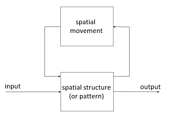
Figure 1: Components of the spatial process and their relationship (source: Rapant, 2014)

Even real-world processes can be classified according to various criteria, e.g. into:

• qualitative (e.g. land-use change) and quantitative (e.g. spread pollutants in water),
• continuous (e.g. soil erosion) and discrete (e.g. earthquakes), etc.

Processes can be modelled only to a limited extent in today’s geoinformation systems. Far more often, there is an integration of geoinformation systems with purpose models of individual processes. The geoinformation system is used for data collection and preparation for the model (so-called preprocessing) and for analysis and visualization of modeling results (so-called postprocessing).

2.2 Modelling in geoinformatics

The real world is represented by the environment that surrounds us. On the contrary, the model world is an “artificial” world, a world that we create based on our observations of the real world. In the first step, we create it purely in our heads - we create a so-called mental model, which represents the real world, the relationships between its objects, phenomena, events and processes, and our intuitive ideas about possible further action and its consequences. We then try to transform it into a computer environment so that the created computer model best captures the observed reality in the context of the tasks we want to solve using the computer model.

We always create each model in the context of its intended use. Therefore, each model is a certain simplification of reality - we capture in it only those aspects of the real world that are essential in the context of the intended use, we neglect the others as irrelevant.

Example (Rapant, 2014): Our task is to create an information system for recording inventory owned by the organization. Looking around the room we are in during the lecture (our real world), only those objects that have an inventory number makes sense to include in the information system. Of the ones listed, they are probably just: tables, chairs, a department, a data projector, a computer, a whiteboard. Everything else is either fixedly connected to the building, and it does not have an own inventory number (windows, doors, lights, sink…), or its price is so low that it makes no sense to record the item (consumable material - chalk, sponge, rag ). Our model world, and therefore our mental and finally computer model, will shrink only on tables, chairs, a department, a data projector, a blackboard. In the context of a given task, this selection of objects is sufficient. Of course, we have completely neglected the phenomena, events and processes that are in the given context is irrelevant.

Thus, we can summarize that the model world is made up of many of models (so far we have mentioned only two - mental and computer), it is simplified and context-dependent.

2.2.1 Modeling of real world objects in geoinformatics

As mentioned in Chapter 1, geoinformatics focuses on the study of properties, behaviour and interactions of spatial objects, phenomena, events and processes through their digital models and using information and geoinformation technologies. Geoinformatics, therefore, works with real-world models. Today, they are based on the first two views of the real world - object and phenomenal.

In this case, we start from an object view of the real world. Geoinformatics here allows you to create real-world models whose central building block is a model image of a real-world object - geographic feature (geo-feature). This can be defined, for example, as follows (Laurini, Thompson; 1994, Rapant, 2014):

A geo-feature is a model image of a localizable real-world object that is indivisible to units of the same class and which is described by geodata.

Let’s take a simple example (Rapant, 2014):

The building of the Rector’s Office of the University of South Bohemia can be an example of a geo-feature, which is no longer possibly divided into buildings, but can be divided into floors, rooms, etc. Other examples are the E55 road, the Malše river, Stromovka, the Zbraslav quarry, the Devil’s Lake, the Prokop coal seam, etc. Note that it is always a specific geo-feature - a model image of a particular real-world object.

Each geo-feature is referred to by a unique identifier, such as an address, parcel number, unique code, etc. Geo-features can represent both real-world physical objects and abstract objects, such as constituencies, statistical units, etc. Although they can be internally composed of more parts, have a unique representation.

We group geo-elements based on the similarity of properties into classes of geo-features. The class of geo-features can be defined as follows (Rapant, 2006):

A class of geo-features consists of a group of geo-features with common properties. Yippee a model image of a class of real-world objects.

Again, we give a simple example (Rapant, 2014).

An example of a geo-feature class can be a building (generally any building), a forest, a tree, a lake, a fault, etc. It is always a general designation of the class of geo-features, not concrete geo-feature. Any of these classes of geo-features is a model image corresponding classes of real world objects.

Geo-feature description components

Each geo-feature, if it is to be adequately represented and processed, must be described in many ways. For geoinformatics, it is crutial to describe the position of a given geo-object in space and its geometric properties. Furthermore, the non-geometric properties of the geo-feature must be specified - the so-called attributes (name, number of floors, porosity, density, depth of deposition…). Last but not least, the description of the geo-object must record its duration and changes over time and its relationships to the surrounding and possibly other geo-feature. We must not forget the description of the operations that can be performed on a given geo-object (or the activities that the geo-feature can perform) and the specification of the description quality that should accompany each description of a geo-feature (Rapant 2006).

The description of a geo-feature by spatial data can, therefore, consist of five basic components (Rapant, 2006):

• geometric - records the position of the geo-feature in space and describes its geometric properties,
• descriptive (sometimes also referred to as thematic) - records non-geometric properties of the geo-object,
• temporal - records the history of geo-object changes over time; it is possible to derive from it the period of existence of the geo-object in the given state,
• relational - describes the relationships in which the geo-object enters with other geo-objects, including spatial relationships with surrounding geo-objects - the so-called topology,
• functional - describes the operations that can be performed with a given geo-object, and as an additional component that does not relate directly to the described geo-object, but to individual components of its description as such is the component:
• qualitative - describes the quality of the geo-feature description.

The following text is devoted to a more detailed analysis of the individual components.

The geometric component of the description of geo-objects is very important in geoinformation systems and must never be neglected; it should always be defined at the required level of resolution and accuracy. There are several areas of problems associated with it:

• the space in which the geometric component is defined,
• determining the position of the geo-feature in this space,
• spatial properties of the geo-object.

For each geo-feature it is necessary to record space, in which its geometric component of the description is defined because it depends on this space how it will be possible to work with the geo-feature. Geo-objects are usually primarily defined in Euclidean space, but there may be situations where they are mainly defined in a topological or other space.

The determination of the position of the geo-object depends on the space in which it is defined. In the case of Euclidean space, the location of the geo-object is expressed directly by coordinates or indirectly by geocode, in the case of topological space by spatial relations to the surrounding geo-objects, etc.

Spatial characteristics of a geo-object include, for example (Laurini, Thompson, 1994):

• length (e.g. a section of road or river, high voltage line),
• area (for example lakes, districts, plots),
• volume (for example, coal reserves or embankment necessary for road construction),
• shape (round, square, elongated),
• irregular shape (for example, cured shoreline),
• orientation (for example the principal axes of the dress),
• centre of a linear geo-feature or area (for example, city centre, the centerline of a road),
• slope (such as a slope).

Measuring these properties is usually simple. The accuracy of their definition depends on the used instruments, procedures and the scale of the base materials. For example, the length of the shoreline of the lake will vary when measured in real conditions by stepping, band, measurement procedures, and will also be different when measuring on maps at a scale of 1: 100,000 or a scale of 1: 1,000.

The thematic component of the description of a geo-feature consists of the so-called attributes (in the narrower sense), which describe the non-geometric properties of geo-features. Each attribute is generally made up of a pair: property name - property value (Frank 1987). The name indicates which property of the geo-object is described by the value. Each geo-object can have at most one value assigned to each attribute (that is, each property).

The values of each property come from a specific domain, which is called a domain. A domain is a potential set of data from which the value of an attribute is selected (Horák, 2011). It can be, for example, the field of integers, the interval on the real axis, or a list of possible values, etc. Different domains are suitable for different properties.

In principle, we can distinguish the following types of domains:

• nominal (enumerated) - e.g. for the type of road it can be (motorway, a way for motor vehicles, 1st class, 2nd class, 3rd class, field, not specified, unknown).
• ordinal (ordinal) - possible values are arranged so that we can compare them (e.g. primordial mountains, Mesozoic, Tertiary, Quaternary),
• interval - e.g. integers from the interval (0, 10), decimal numbers from the interval (0.5, 14.0), values can be added, subtracted, their difference is interpretable; however, the scale does not have an absolute zero, so they cannot be measured; an example is a temperature given in \(^{o}\) C),
• proportional - any scale having absolute zero, e.g. percentage, temperature expressed in \(^{o}\) K, etc.; these values can also be measured.

Each geo-feature can have a maximum of one value assigned to each property.

Time component of the geo-feature description

Geographers and historians emphasize that it is necessary to take into account not only spatial but also temporal aspects (i.e. both position in space and “position” in time) of objects, phenomena, events and processes in the real world for their properly understanding (Gregory 2002). However, most commercially available programs for the creation of geoinformation systems today cannot work with time in a full-fledged way. It stems from the fact that the inclusion of time in the data model brings many conceptual problems, which so far represent a specific obstacle that is difficult to overcome. If the user needs to work with time, it is up to him to solve this problem himself at the level of the data model of his application.

Unfortunately, the complexity of current and systematic processing of space and time aspects of real world objects, phenomena, events and processes is so significant, that we usually have to compromise: either we prefer spatial dimensions, we record them in great detail in the whole area of interest, but we then have to significantly simplify the record over time (i.e. we can not record the development in time) or we prefer time aspects (i.e. a detailed history of the development over time) and then we must either significantly reduce the spatial extent of the studied area or considerably reduce the detail of the recorded spatial aspects.

Pequet (in Gregory, 2002a) states that a full-time geoinformation system should be able to answer three types of queries:

1. For changes in real world objects, e.g. Has the real world object changed its position in the last two years?, Where was the object a year ago? Or How has the object changed in the previous five years?.
2. For changes in the spatial distribution of buildings, e.g. Which lands that were used for agriculture on 1 January 1990 were converted into area intended for civil construction by 31 December 2000? Or How were areas designed for commercial development activities distributed to 31.12.1995?.
3. On the time course of several geographical phenomena, e.g. In which areas did landslides occur within one week after the occurrence of torrential rains?.

The time differs significantly in nature from the geometric and descriptive properties of a feature. Perhaps mainly because it cannot be understood as a component of the description itself, but always in close relation to the components mentioned above of the geo-feature description (Fig. 2). Series of versions of the geometric and thematic elements of the geo-features description serve for temporal changes recording.

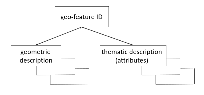
Figure 2: The relation of time to the geometric and thematic component of the description of a geo-object. Changes over time are captured here by individual versions of the geometric and thematic description (source: Rapant, 2014)

Relational component of the geo-feature description

Individual real world objects can enter into mutual relations with other real world objects. However, some of these relationships can be derived from data (they are expressed implicitly), other relationships must be specified explicitly, such as ownership relationships. The relational component of the geo-feature description focuses on the description of these relations.

Relationships between real world objects can be:

1. topological,
2. time,
3. metric,
4. syntactic,
5. is part-of,
6. others (e.g. proprietary).

Topological relations

Table 1 contains examples of spatial relationships as we encounter them in the real world.

Table 1: examples of spatial relationships

relationship	typical example
belongs to …	the village belongs to the district, section el. management belongs to a continuous network of higher-order
contains/consists of	the state is composed of regions, these include municipalities
located in	the building is located on a specific plot
boundary	the two parcels have a common border

While in most analogue maps most of these relationships are included implicitly, the user perceives them intuitively, in digital maps they must be expressed explicitly because the computer has no intuition. Computer processing of geo element relationships, therefore, requires additional information describing these relationships or requires instructions explaining how this information can be obtained directly from the data.

Besides, some of the relationships of geo-features can depend on the specific state of the displayed reality. For example, in distribution networks, the state of the valves can determine which parts of the networks can be considered as one logical unit. In such a situation, it is necessary to distinguish between still current and potential relationships.

Example (Rapant, 2014): Let’s have a gas pipeline and examine the interconnection of two areas, i.e. whether they are topologically interconnected. A gas pipeline passes through these areas. This pipeline includes a slide which allows interrupting the flow of gas through it. If the slide is closed, the current topological relationship between the areas is “unconnected”, and the potential topological relationship is “connected”.

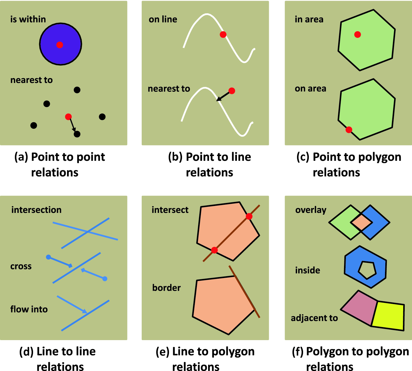
Figure 3. shows examples of topological relationships between geo elements of different dimensions.

Time relations of geo-objects can be as follows (Rapant, 2014):

• random co-occurrence - geo-object occurs completely randomly, has no explicit causal relationship to other geo-objects (for example, field and stream),
• coexistence relationship - geo-objects coincide with other geo-objects (e.g. the existence of a car park links to the presence of an access road),
• successive (subsequent) relationship - geo-object occurs with a time lag after its origin another geo-feature (e.g. so-called brownfields, which arise after the end of production in the industrial zone),
• causal relationship - the geo-object arises as a direct consequence of the origin of another geo-feature (the water surface will be created as a result of the formation of a terrain obstacle - an artificial dam, damming the valley by landslides, etc.).

Metric relations mainly include the direct mutual distance of geo-objects. These relationships are not expressed explicitly, and they are usually derived directly from the geometric component of the description of geo-objects using the metrics of the selected space.

Syntactic relations

The syntax generally expresses which geo-objects can (or in some cases even have to) have a topological relationship with each other and possibly also a metric and temporal relationship, and which, on the contrary, must not have a specific relationship.

Examples (Rapant, 2014): Intersection of two roads: there may be an intersection of two motorways resp. highways and first-class roads, but there must be no intersection of highways and roads second or third class, etc. The pump must always be on the road, it cannot stand outside, without being connected to the road network. A river can flow into another river, lake or sea, but certainly not into a motorway, for example.

The relation “is a part” expresses the composition of geo-features. For example, a republic consists of regions, i.e. a region “is part of” the republic. We assume that the composition of all areas together will create a whole republic (complete coverage) and that the regions are mutually disjunct (do not overlap).

This type of relationship partially overlaps with topological and possibly syntactic relations, but this may not always be the case.

Example: We can easily demonstrate the use of different species at the edges relationships:

• topological relations say which region is adjacent to which,
• syntactic relations say that a county can generally be adjacent to another province or with another state,
• the relationship “is a part” means that the region is part of the country, individual regions are disjunct, and all regions together cover the territory of the whole state.

In the category other relationships we can include all links that do not concern space or time. These may include, for example, ownership relations, relations of superiority and subordination, relations of membership, etc. These relations are expressed explicitly.

In general, we pay only a small amount of attention to the component of the description of geo-feature relations (except of topology, of course), so its more detailed elaboration is a question of a somewhat near future. In geoinformation systems, this component is usually implemented within a data model.

Functional component of the geofeature description focuses on the description of operations that can be performed with the geo-feature. These operations usually lead to a change in the state of one or more components of its description (and thus to a change in the state of the geo-object as such).

Examples of these operations are:

• change of ownership of the real estate,
• construction of a new house,
• demolition of the house,
• reconstruction of the house,
• replacement of the municipality’s affiliation to the district,
• change of the name of the village,
• connection of two townships,
• change of distribution network management,
• blocking the implementation of any changes,
• unblocking the application of any changes, etc.

These operations describe real-world events. They, therefore, represent what actions must precede the achievement of the new state. Their exact description is equal to the description of the behaviour of a real system.

Example (Rapant, 2014): Let’s have a plot. Let’s say that the allowed operations with a plot are:

• merger of two plots,
• parcel division,
• change of parcel owner.

If someone wants to perform another manipulation of the plot, for example, move to another location, this operation will not be accepted.

The general conclusion for this component is generally the same as for the previous element. Today, not enough attention is paid to it on its own. The only exceptions are perhaps only object-oriented systems.

In geoinformation systems, this component of the geo-object description implements through program code that manipulates the geo-object to achieve desired condition.

Qualitative component of the geo-feature description, metadata

The data contained in spatial databases are generally multidimensional. And the errors of this data have the same (multidimensional) nature. It follows that a simple index cannot describe the error in determining a particular spatial data.

E.g. spatial accuracy includes both horizontal and vertical components, which cannot always be separated. Thematic accuracy depends on the type of data (e.g. numerical or categorical) and often on spatial accuracy. Time accuracy is an essential but often overlooked dimension of spatial database accuracy. And the accuracy of the description of relationships and operations is still not talked about at all.

Data reliability is often (though not always) an inverse function of their age because all components of a geo-feature description can change over time. Also, descriptions of geo-objects obtained in earlier times using earlier methods often have (at least from today’s point of view) limited or even unknown accuracy.

The quality of a geo-feature description is usually documented by the following parameters, called metadata (Horák 2002):

• the accuracy of the geometric component of the geo-feature description, often defined
  • accuracy of the horizontal component,
  • accuracy of the vertical component,
• the level of resolution (e.g. whether the watercourse will be represented by one line, copying the centre of the stream, or will be represented by two lines, copying both banks),
• the extent of geographical coverage,
• by way of representation (discrete vs continuous),
• the accuracy of the thematic component of the description of geo-objects, usually defined by accuracy individual attributes,
• the accuracy of the time component of the description of geo-objects, usually defined by:
  • up-to-dateness of individual components,
  • update interval,
• logical certainty between geometric and descriptive component,
• completeness, given
  • completeness of data,
  • completeness of the model,
  • completeness of attributes,
  • completeness of values,
• relevance of the geo-feature description (for which operations the geo-feature description can be used, or for which it is not).

These parameters can be monitored either at the level of individual geo-objects, if any justified, or rather at the level of groups of the same geo-objects (for example, for all roads targeted in the same period by the same method, one set of these parameters will be defined), usually included in so-called data sets. A combination of both approaches is also permissible. Dataset can be defined as follows:

A dataset is an identifiable collection of data.

Today, this component of the description of geo elements is discussed relatively intensively, mainly in connection with the construction of so-called metadata services, which are to provide users with information about the existence of individual data sets and the metadata is descriptive. The user can then quickly decide based on the provided data, whether the searched data set is suitable for his needs. Because metadata usually also contains data about the provider of the data set, the user can address it directly in case of a definite conclusion.

2.2.2 Modeling of phenomena in geoinformatics

To model real-world phenomena, geoinformatics uses some different so-called networks, the basic building block of which is usually cell, representing a defined part of the real world space and carrying the values of the observed Properties. The most commonly used is a regular network of square cells called a raster.

We know rasters from digital photographs. Here, each cell of the raster (in this case we are talking more about pixels) is assigned a colour taken from the scanned space and by perceiving the whole raster we create in the brain the perception of the image of the scanned reality.

We proceed similarly for the raster. We assign a value of the monitored property (e.g. room air temperature) to each raster cell. If we looked at only numerical values, it would be difficult to get an idea of the temperature distribution in space. Therefore, when visualizing the raster, we use a similar principle as in digital photography. We will find the minimum and maximum value of the monitored property in the raster and create a conversion colour scale, which will allow each numerical value to be assigned a specific colour shade. Its will convert the matrix of numbers into a colour image, the perception of which will enable us to immediately get a perfect idea of the distribution of air temperature values in space.

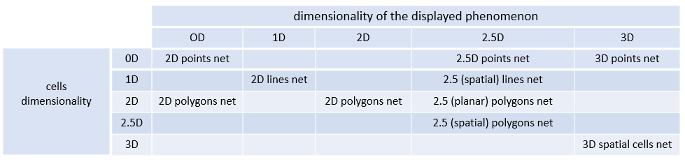
Table 2 shows possible combinations of the dimensionality of the displayed real-world phenomena, cells used for its representation and the dimensionality of the resulting cell network (Rapant, 2006).

Cell network description components

Each cell network, if it is to represent a given real-world phenomenon correctly and if it is to be properly processed, must be described from several points of view:

• On the one hand, we must have information on the properties of the displayed phenomenon,
• further information about own cell network and
• on network cell properties.
  

Description component of properties of displayed phenomenon

Each displayed phenomenon of the real world must be described from practically the same points of view as in the case of geo-objects. It means that even here we work with the following components of the description of phenomena:

• geometric,
• thematic,
• time,
• functional,
• relational,
• qualitative.
  

The following problems are associated with the geometric component of the description of a real-world phenomenon:

• the space in which the phenomenon occurs (and described) and its dimensionality,
• spatial continuity of the phenomenon,
• spatial definition of the phenomenon.

Space - in this case, we are interested in what space the phenomenon occurs, how many dimensions this space has and how the phenomenon is distributed in it.

Spatial continuity describes how the values of the properties of a given phenomenon change when the position in space changes. In general, we recognize continuous phenomena, when the values of the observed properties change continuously with a smooth shift in position, and discrete phenomena, when the values of properties change by a jump and possibly for some areas of space are not even defined.

Spatial delimitation basically indicates the boundaries of the studied phenomenon in space.

The thematic component of the description of the phenomenon includes information on the non-geometric properties of the displayed phenomenon, i.e. enumeration and description of these properties, description of their types, etc.

Time component describes the behaviour of the displayed phenomenon over time and possibly characterizes the dynamics of its development (speed and frequency of changes, etc.). We distinguish phenomena:

• static,
• dynamic.
  

Relational component describes possible dependences of the displayed phenomenon on other phenomena, objects and processes of the real world.

Functional component - the subject of this component of the description are operations applicable to the given phenomenon.

Qualitative component characterizes how high-quality information we managed to obtain within the compilation of previous components of the description of the displayed phenomenon.

Description component of network properties

The network property description component describes the network used to represent the displayed phenomenon from the following points of view:

• network size,
• network type,
• network size,
• method of assigning property values to cells,
• Interpolation rank within the network.
  

Network size describes the number of network dimensions - usually 2D, 2.5D or 3D network.

Network type describes whether the network is regular (composed of cells of the same dimensions and shapes) or irregular (cells of different sizes and shapes).

Network size is important, especially in the case of regular networks, where the number of cells in the direction of individual dimensions and possibly the total number of cells should be described. In the case of an irregular network, this description will be more complicated and will depend on both the characteristics of the network and the agreement or standard adopted. It can also be specified explicitly by the network boundary.

How to assign property values to cells describes how to determine the value of each property of the displayed event that will be assigned to a cell.

Interpolation of values within the network - description of the interpolation mechanism used for interpolating values of the network, i.e. calculation of values of a given property of the displayed phenomenon for cells to which the value of this property has not been assigned.

Cell property description component

This component can exist in two forms, depending on whether the network is composed of cells with the same properties or not. In the first case, a single description applies to all cells of the network; in the second, each cell has its own description. In each case, however, the following aspects should be affected by the properties of the network cell:

• cell size,
• cell shape,
• cell size,
• interpolation rank within a cell,
• cell coordinates.

Cell size describes the number of cell dimensions - in this case, all options from the range 0D to 3D come into consideration.

Cell shape describes the shape that a cell has. It can be either regular or irregular and can be further characterized by a specific pattern, such as a point, line, circle, hexagon, cube, etc.

Cell size describes, for example, the length of the side of the regular shape or the length of individual lines forming the cell boundary and the angles subtended by them (in the case of an irregular cell bounded by straight sections of the boundary), etc.

Interpolation of values within a cell - in some cases (e.g. digital relief models) the values of the properties of the phenomenon are not considered constant within the cell. Still, they are derived by interpolation from values related to, e.g. cell vertices. In this case, it is necessary to establish an interpolation mechanism that allows the values of these properties to be derived anywhere on the cell surface.

Cell coordinates - this describes either the method of deriving the coordinates of any cell (in the case of a regular network) or the coordinates of the cell to which the description relates (in the case of an irregular network).

2.3 Space in Geoinformatics

It is complicated to define the concept of space. The idea of space is comprehensive, ranging on the one hand from real physical space (that is, space that we know from our everyday experiences) to abstract space on the other. It is commonly defined as a set of elements that has some distinctive features of real physical space. It is common for a person to work with different conceptions of space and to switch between them usually and without difficulty. He can thus choose the concept of space that best corresponds to the task. For example, if we need to determine the area of the plot, we will work in the so-called Euclidean space. Solving problems such as finding a suitable route for driving between two cities by road, we will work with an area where we are interested in which cities are connected by roads. Still, we do not have to care about knowing the exact location of towns and roads. In this case, we will work in the so-called topological space and we will use the tools of graph theory.

Although these different conceptions of space are used in everyday life without the need for their formal description, formalization is necessary for the transition to the environment of computer-oriented information systems (Kolář 1997).

2.3.1 Historical development of the concept of space

From the point of view of geoinformatics, the idea of the duality of the concept of space as is very important continuous field resp. sets of discrete objects. In practice, we look at space in two ways (as a):

1. continuous space which consists of an infinite set of places (or also a set of points) to which the values of the observed (non-geometric) properties of this space relate,
2. discrete space formed by a (finite) set of real-world objects that have explicitly expressed their position in space, geometric properties, topological relations and only to these real-world objects are non-geometric properties related (Figure 4).

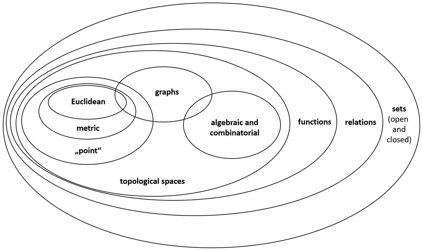
Figure 4: Hierarchical division of mathematical spaces (source: adjusted according to Rapant, 2014)

The duality of our conception of space has a fundamental impact on geoinformatics and spatial modelling and analysis in general. It is reflected, among other things, in the representation of space in geoinformation systems, where two basic approaches are commonly used (Gahegan, 1995 in Rapant, 2014):

• space is defined as a set of places to which non-geometric properties are assigned (i.e. the concept of “continuous” - field), or
• space is defined as a set of objects (i.e. the concept of discrete - objects) having spatial properties (such as shape, position, topology, etc.) as well as non-geometric properties.

These two different approaches have a direct impact on the representation of the real world in geoinformation systems.

2.3.2 Mathematical spaces

Figure 4 schematically shows the hierarchical division of mathematical spaces, as shown in work (Albrecht, Kemppainen 1996 - in Rapant, 2014). At the lowest level, there is the concept of spaces as sets of objects that are without any internal structure. Within these sets, only simple membership-type relationships can be defined.

A subset of spaces that allow us to define relationships between two or more sets stands at a higher level. We use this rather simple conceptual model of space when working with relational databases. A subset of the conceptual relation space is the function space, which allows us to transform each member of the first set into a member of the second set.

Topological spaces, again one step higher, approach the concept of space perceived by humans for the first time. Looking at Figure 4, we can easily find that topological spaces consisting of two primary groups: point and algebraic. While the topology of points works with the notion of neighbourhood, algebraic topology is the basis of graphs.

If we introduce distance into this space, we get into a subset of so-called metric spaces. Metric spaces must meet certain conditions, relating to distance measurements. Euclidean space, standing at the top of our hierarchy, introduces the last important feature, and that is direction.

The concept of space in geoinformation systems is not simple and makes full use of the above indicated width. These systems commonly work with a variety of spaces. The most basic of them is the space in which the geometric properties of geo-objects are defined. It is closest to real physical space. It is almost always a Euclidean space. The geometric properties of geo-objects are described in it using a suitable coordinate system.

One of the primary purposes of geoinformation systems is to perform spatial analyzes. These analyzes do not necessarily have to be completed in the same space that is used to define the geometric properties of the geo-objects. An example is the analysis of the type Find the shortest route in the road network from place A to place B. For such analyzes, we do not even need to know any coordinates, we only need to know the so-called road network topology. Thus, with our spatial analyzes, we get into topological space, where there is no coordinate system and distances are not measured here.

And it would be possible to continue with other examples of spatial analyzes and their corresponding ones premises.

The above facts can be summarized as follows:

Geoinformation systems work with different spaces. One of them can be considered fundamental, and that is the space in which the geometric component of the description of geo-objects is defined. It is mostly an Euclidean space. Furthermore, there are several of other spaces in which spatial analyzes are performed and in which the results of these analyzes are provided.

Topological space

Topology is a mathematical discipline that studies the mutual spatial relationships of geometric objects. It is typical for a topology not to work with the coordinates of these objects. It is also sometimes called rubber sheet geometry (Herring 1987 - In Rapant, 2014). It studies the spatial relationships of objects that can be defined independently of the coordinate system. It, therefore, works with the so-called ** topological space **. In the field of geoinformatics, the term topology usually refers directly to the spatial relationships of geo-objects.

For geoinformatics, topology as a mathematical discipline is of particular importance: with its help, it is much easier to analyze and visualize different types of systems, such as cadastral maps, complex ecological conditions, transport and engineering networks, etc. (Streit, 2000). In geoinformatics, by default, we work only with the topology of at most two-dimensional geo-objects, represented by points, lines and polygons. Solving the topology of three-dimensional geo-objects is still too difficult to handle in a reasonable amount of time, even with today’s relatively powerful computers.

In every modern geoinformation system, there is knowledge of the topology of recorded geo-objects necessary prerequisite for successfully managing user requirements. E.g. if he has geoinformation system to provide an answer to the question Which plots are located around the road XY in the village Z? or What is the area of forests situated in a radius of 100 km from the considered construction site of a new pulp mill? geo-objects necessary.

Examples of spatial relationships of geo-objects are in Table 3 and Figure 3. In principle, the spatial relationships of points, lines and polygons are solved. See topological rules in the ArcGIS geodatabase.

Table 3: Examples of spatial relations between/among geofeatures (source: Rapant, 2014)

feature(S)	topological relationship to other features
the point lies	at the endpoint (node) of the line - coincidence
the point lies	at the boundary of the polygon
the point lies	inside the polygon
the point lies	outside the polygon
line	does not cross itself
line	touches a polygon
line	intersects the polygon
polygon is	simple/complex
two polygons	touch
two polygons	intersect (overlap)
two polygons	are disjunct

Metric spaces

In metric spaces, you can measure distances between any points in space. Different regulations for measuring distances (so-called metrics) can be introduced in different spaces.

Metrics must generally meet the following conditions:

• \(d(A,B)\geq 0\) … the non-negative condition of the distance,
• \(d(A,B)=0\) just if \(A = B\) … the condition of identity,
• \(d(A,B)=d(B,A)\) … symmetry condition,
• \(d(A,B)\leq d(A,C)+d(C,B)\) … the condition of triangular inequality.

A set \(M\) with such a metric \(d\) is called a metric space, which we call \((M, d)\). The elements of the set \(M\) are called points and its subsets of point subsets. The metric is basically a generalization of the term distance, and therefore the number \(d(A, B)\) is also called the distance of the points \(A\) and \(B\). On the same set of points \(M\) we can define different metrics; if the metrics \(d\) and \(e\) are different, then the metric spaces \((M, d)\) and \((M, e)\) are also different.

Two metrics are most often used In the environment of geoinformation systems:

• Euclidean, designed for measuring distances in spaces with continuous coordinate systems,
• Manhattan, designed for measuring distances in spaces with discrete ones coordinate systems and in spaces where it is only possible to move along two mutually perpendicular networks of parallels.

The Euclidean metric (also Euclidean distance - Figure 5) is defined by:

\(d_{ij}=\sqrt{(x_{i}-x_{j})^{2}+(y_{i}-y_{j})^{2}}\).

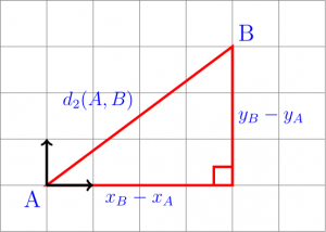
Figure 5: Euclidean distance (source: https://dr-apeiron.net/doku.php/fr:vulgarisation:distance)

Another way to measure distances was proposed for the city of Manhattan. This city is known for its almost consistently rectangular network of streets. From a taxi driver’s perspective, distances in this Manhattan space can be measured using the Manhattan metric defined by the relation (Maguire et al. 1991)

\(d_{ij}=|x_{i}-x_{j}|+|y_{i}-y_{j}|\).

Manhattan metrics are suitable for measuring distances in densely populated areas (such as some neighbourhoods in our cities).

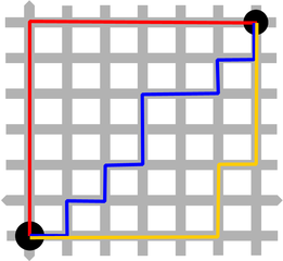
Figure 6: Manhattan distance (source: https://commons.wikimedia.org/wiki/File:Manhattan_distance_bgiu.png)

The conditions for metric spaces do not apply in all spaces with which geoinformation systems work in spatial analyzes. For example, when expressing time availability in network tasks, the symmetry condition would assume that the uphill travel time is the same as the uphill travel time. Similarly, the invalidity of a triangular inequality can be proved. As a result, it is generally not possible to subtract travel times between any pair of points from time availability maps, but only between the start and any location, with the reading being valid only for driving from the beginning to the selected location. If we were interested in driving time in the opposite direction, we would have to generate a new map starting at the second of the pair of points. Therefore, such a “time” space does not belong to metric spaces.

Euclidean space

Euclidean space is a mathematical abstraction and extension of the “ordinary”, usually three-dimensional space in which our daily lives take place. Euclides was the first to deal with it about 300 BC. He compiled a system of postulates and definitions, from which theorems of geometry were derived, which have been used since time immemorial by meters, designers, builders.

In the 17th century, Descartes (1596-1650) introduced a rectangular coordinate system into Euclidean space (we call it the Cartesian coordinate system), thus enabling the connection of geometry with arithmetic and algebra. It paved the way for the generalization of Euclidean space to more than three-dimensional cases.

\(N\)-dimensional Cartesian coordinate system in the \(n\)-dimensional Euclidean space \(E_n\) consists of \(n\) mutually perpendicular coordinate axes that intersect at a common origin and use the same units of measure.

Each ordered sequence of \(n\) real numbers \((x_1, x_2, \dots, x_n)\), where \(x_i \in \mathbb{R}\), defines exactly one point in this coordinate system (and thus in Euclidean space). A metric for measuring distances is defined in Euclidean space. So it’s a metric space.

Euclidean space can also be defined as a set of points \(M\) representing sequences in \(n\)-dimensional Euclidian space formed by a Cartesian product (more precisely, a Cartesian power defined over a set of real numbers \(\mathbb{R}\)). Vectors in \(n\)-dimensional Euclidian space are then called coordinates of points of the set \(M\).

We describe our real world as a three-dimensional Euclidean space (\(E_3\)); however, to display in geoinformation systems, we usually convert it to a two-dimensional \(E_2\) space. We use many of techniques to do this, called cartographic representations (see below).