6 Database systems for GIS

6.1 Approaches to data processing on computers

6.1.1 Agenda file processing

The first computer data processing systems were developed to provide a well-defined set of functions for use with a specific set of data. The data was stored as one or more computer files that were accessed using software specialized for this purpose. Such an approach is called agenda file processing.

Agenda file processing is suitable for some specific purposes, but for others it has serious shortcomings. Every application user program must directly access each data file it uses, it must know how the data is stored in each file. This is a source of significant redundancy, as instructions for accessing data files must be present in every application program. If the structure of the data file is modified, the access instructions in all application programs must be modified or vice versa.

• Redundancy: imagine, for example, how many times and in how many files the names and addresses of residents (registry, building authority, etc.) can be stored within one city office. Such duplication leads to a waste of inputs and computing power.

Another serious problem occurs when sharing data with different, different applications and users. In this case, there should be some overall control over which users would be given access to the data and which would determine what changes they can make to the data. The absence of such control seriously compromises the integrity (and quality) of the data. Thus, when data is shared by multiple applications and users, their integrity, independence, and security are lost.

• Insufficient data integrity: Where data is stored more than once, there is a possibility that individual copies will not be identical. For example, one survey at a local authority found ten copies of a “final” trail map, each stored in a different department, containing different trails, and only one of which was regularly updated. Citizens tend to consider authorities and organizations as unified units, ie if Ms. Nováková becomes Ms. Horáková and informs the housing office about this happy event, she will probably not be too thrilled if the Tax Office sends her letters in the name of Ms. Nováková.

other problems associated with agenda data processing:

• high maintenance costs - application programs tend to have an individual (sometimes even eccentric) style, because they often work in different operating systems and are written in different languages, organizations must have application specialists to maintain them
• lack of identical interfaces - different applications can come from different sources and therefore have different user interfaces, the result is a low probability that the applications will work together
• Ad hoc “enhancements” - application programs are usually adapted to meet the requirements in force at the time of the award of the contract for the software concerned. However, as organizations evolve, application requirements may change and a number of ad hoc “reports” may be created to extend application programs to new areas.
• data sharing issues - because agenda file processing focuses on applications, some applications tend to affect data structures, making it difficult for other applications to access that data
• lack of data standards
• insufficient protection - where there are multiple copies of files, with little degree of central control, there is always the possibility that data considered confidential will be released into circulation
• lack of common concept and insight - application-oriented concept makes it difficult to ensure that information retention and computer systems evolve in a way that is optimal for the organization (as opposed to what may be optimal for individual departments within the organization).
  
  

6.1.2 Database conception

The above-mentioned problems of agenda data processing are solved by the so-called database approach to data processing. In this case, the data is stored in a structured database, which is managed by a database management system (DBMS), which contains a set of programs whose task is to manipulate and manage the data in the database. These programs have been designed to ensure the integrity of the managed database. The database is designed to minimize its redundancy, ensuring the independence of application programs on the form of data storage. The DBMS thus acts as a central, central control over all interactions between the database and the application programs through which users use it. The services provided by DBMS also significantly simplify the development of new application programs and the usability of data.

Database management system requirements:

• data access for all applications without multiple storage * simultaneous data access for multiple users,
• various search methods,
• data protection against unauthorized access and against hardware and software errors,
• resources for central data management,
• application independence of data,
• possibility to create even complex data structures,
• hiding the mechanism of structures and data storage.
  
  

6.2 Database design

Figure 1 presents a simplified model of the process that a database project goes through from its inception to completion.

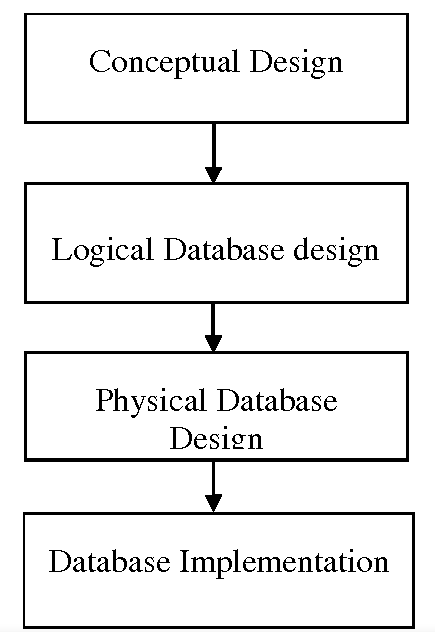
Figure 1: Phases of database design (source: https://www.geeksforgeeks.org/introduction-of-3-tier-architecture-in-dbms-set-2/)

Preliminary analysis includes cost-benefit analysis, feasibility studies, system analysis, determination of user needs, etc. The decision to continue building the database follows the work of the database designer who creates the logical design. The designer must thoroughly get acquainted with the structure of the data used and then create a conceptual data model (identification of entities, relationships between entities, attributes of entities), which will become the basis of the database itself. The conceptual data model thus represents a logical list of entities, attributes and relationships between entities that the database will contain. It is designed to be independent of any software program. Its purpose is to provide a “simple” overview of what the data structure in the created database should look like.

If the logical design is successfully completed, the next stage that follows is the translation of this design into the selected DBMS software (the design is “mapped” to the software). This phase includes the establishment of a data structure - record structures, field and file names, indexes and algorithms that will represent the conceptual design within the DBMS software.

Once the physical design of the database has been created, the next step is to ensure that this design actually works, ie that it provides the outputs required by the user. So the testing phase begins. This is followed by the implementation phase, when operational data is entered into the database, documentation for users is compiled and they are also trained. Because database organizations never stop evolving, database requirements evolve with the organizations that the databases serve. Therefore, the last phase is not negligible - updating or expanding databases, their maintenance.

6.2.1 Database models

According to Scheber (1988), a data or database model is a system of modeling tools used in modeling. The result is a specific data organization, representing a slice of reality.

The development of database systems went from the network, through the hierarchical to the most widespread relational model, to the object-oriented model developing today:

1. hierarchical model - entity types are strictly mapped in this model on the example of the father-son relationship. The structure is formed as a system of joining all records in the form of a tree. The top of the hierarchy is the root. Hierarchical model only 1: 1 and 1:n relationships between individual entity types. Connections exist only between superiors and subordinates, there are no connections at the same level (one of the biggest disadvantages of this model). If an m:n relation exists in the hierarchical model, we must represent it as an \(m\)-multiple of the 1:n relations. The big disadvantage of this model is the high redundancy (repeated storage of the same data in different places) and the specified query procedure, given by the hierarchy, which is difficult to change. Hierarchical structures are characterized by a high search speed, are easy to understand, and are easy to update. This type is used, for example, in administration, for bibliographic databases or reservation systems in transport.
2. network model - omits from a strict hierarchy and there may be m: n relations in it. It can therefore be understood as a kind of generalization of a hierarchical model. Its structure is more flexible and less redundant than hierarchical. Much more extensive information about the links between records must be stored, which increases the size and complexity of the data files. Managing this added link data is relatively time consuming. On the one hand, this model is more flexible, on the other hand it becomes complicated and chaotic. It is used, for example, when searching for the best connection in a communication network. Note: Hierarchical and network structure are sometimes referred to as navigation, because the links in them are constructed using search engines (pointers), which are also used in the design of application programs.

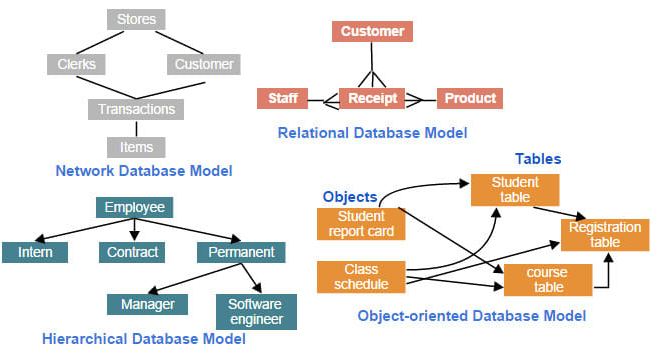
Figure 2: DBMS models (source: https://www.fiverr.com/arujfatima/create-sql-database-and-design-database-model)

3. relational model - its concept first appeared during the 70s, it is based on a mathematical approach - relation. He was motivated by the effort to describe data in their “natural” form and to eliminate the need to create application programs over the database with a detailed knowledge of the data storage format. Compared to the above, it excels in simplicity. The basic and only structure is a table (session) in which data is stored. Therefore, relational databases are sometimes also called table databases. In the table, each row corresponds to one element (record). The values of individual attributes (item) are stored in the columns. Each table is usually stored as a separate file. Data redundancy is much lower here than with the hierarchical and network model. In this model, there is no hierarchy of fields inside the record, each field can be a key to access data in a different table. Because there is no address data in the tables, searching for records or fields is sequential, so it is slower than in a hierarchical or network model. The degree of a session is the number of their attributes. All possible associations (1: 1, 1: n, m: n) between entity types are represented by keys. A key is generally a unique attribute or combination of attributes. Keys have two important roles in a relational data model:

• serve as search engines between different sessions, ie they connect a table with another table,
• serves for unambiguous identification of entities - so-called primary keys (it must have two properties: it is unambiguous, it is minimal - it is not possible to omit any attribute in order not to violate the rule of unambiguity).

Operations that can be performed with sessions are divided into two basic groups:

• relational algebra,
• relational calculus.

Database storage and retrieval operations are based on rules and functions defined in the mathematical theory of relational algebra. Searching for attributes that belong to each other and are stored in different tables is performed by joining tables that contain the same key value. This procedure is called a relational link. The link creates a new table from the data of the selected tables, which can only remain virtual and does not have to be physically stored in the database. There is no limit to the type of data retrieval command. Relational algebra includes unification, intersection, set difference, symmetric difference, and Cartesian product.

By unifying the sessions, we create a new table that contains all the rows of both input tables. If these tables have some rows identical, they appear only once in the output table. Intersect we will create a table that will contain only rows identical for both input tables. By a set difference, we create a table in which all rows of the first input table will be, but only those that do not occur in the second table. With a symmetrical difference, we will create a table in which all rows of both tables will be, except those that occur in both tables at the same time. The Cartesian product creates a new table by joining rows from both tables by each system.

Relational calculus operations include projection, selection, and joining. The projection creates a new table by selecting the specified columns from the input table. All duplicate rows in the created table are then deleted. The selection creates a table with the same header as the input table, but a smaller number of rows. Rows are selected according to an attribute whose values are compared to another row or constant. We can understand a connection as the creation of a certain subset of the Cartesian product of input tables. Unlike the Cartesian product, a join of two tables is performed only if the defined condition for the join is met. This is an expression in which two attributes from both input tables are compared.

The tool for achieving a better data structure is standardization. The goal of normalization is to refine the image of reality in data. It is basically an attempt to maintain consistency between the conceptual and logical data model roughly according to the rule “one record for each object”. Such records are then referred to as normalized. In practice, the first three normal forms are especially important. There are other normal forms.

A non-standard record can often contain one or more groups of items that are repeated and not part of the key.

4. Object-oriented model - based on 5 principles, derived from experience with other types of logical data models:

• Each entity is modeled as an object with its own identity, which is provided by an object-oriented database system (OODBMS).
• Each object is encapsulated, ie protected against the environment and has its own structure (attributes) and its own behavior (methods), ie. that the object is functional (we do not have to be more interested in its internal procedures, but only in its behavior towards the environment).
• Objects communicate with each other using messages (if an object receives an understandable message, it responds to it in the planned way).
• Objects with the same attributes and methods create object classes, an individual object is called an example.
• An object class can be divided into specialization subclasses (derived classes) that inherit the attributes and methods of the superclass (superclasses).

Recently, the need to use and implement this approach in structuring information in general, but also in GIS, has been much discussed.

6.3 Geographic database organization

Because both spatial (geometric) and non-spatial (attribute) data are stored in a database, the problem of data organization in GIS is considered a “database” problem. Spatial data are represented in GIS by storing the geometry and its associated attributes. The individual GIS systems differ considerably in terms of the way data is stored and the way in which attributes and the spatial (geometric) part of the geographical database are interconnected. Based on these differences, a simple typology of GIS systems can be created:

1. GIS of “first generation” (without DBMS)
   1. systems without attribute files - purely raster access does not allow separation of location data and attributes (space is divided into regular network, each cell contains attribute value, corresponding cell location, each raster map stored as a separate file) - e.g. “MAP” family of systems GIS.
   2. flat file systems - separate storage of geometric and spatial data in separate environments and their connection only when needed - object geometry is stored in a special environment together with an identifier that provides a connection to the space where attributes are stored. An individual object (individual geometry) can have only one identifier, but more attributes. To obtain information about objects, it is necessary to enter both environments. The most basic form in which attribute data can be stored is the use of so-called flat files, which are simple tables. The disadvantage of this method of storing geographic data is the different standard for storing geometric and attribute data, because each system has its own format. Some authors (eg Maguire, Goodchild, Rhind, 1991) refer to this data storage strategy as a “hybrid concept” and consider it obsolete.
2. GIS of “second generation” (with DBMS system) - separate storage of geometric and spatial data in a single database - geometry and attributes are stored in a single database as separate files. This method of data storage is used by most common current GIS. Storing topological information causes certain problems. This method is sometimes referred to as the “enhanced DBMS concept”. The main dividing criterion between these systems is that some of them use relational DBMS only to store attributes and prefer their own spatial data management software, while others use RSBD to store both geometric data and attributes. The first group is referred to as dual systems, the second as integrated architecture systems.
   1. dual systems - ARC/INFO, MGE and Geo/SQL systems are examples of GIS systems that support dual architecture and use the purchased DBMS software for attribute management and its connection with its own program that manages spatial data. The model architecture of dual systems is shown in Figure 3. Due to their duality, these systems can have problems with data integrity and also have problems with seamless data (database divided into map sheets, which brings problems mainly in terms of maintaining topology in the model).

2. integrated systems - systems that integrate into the common structure of RSŘBD both spatial and attribute data - e.g. SYSTEM 9, SDE (Spatial Database Engine), GeoMedia or ARC/INFO with the ArcStorm module - so that these programs can store spatial data in the system DBMS, had to overcome a number of difficulties associated with the nature of spatial data, which was solved in practice by using a superstructure to the basic relational model. Data management is therefore taken care of by middleware, which is a product that forms the communication layer between the database and GIS SW, not the database itself. Thanks to the storage of the spatial part in the database, it is possible to work with seamless spatial data (there is no need to divide the space into map sheets). The disadvantage of the model is its relative slowness, due to the fact that relational databases cannot efficiently store spatial data. These systems can also have data integrity issues.

Figure 3 shows common method for linking attributes to spatial entities that have unique identifiers in geographic data files, and these identifiers are also used as primary key values in relational tables. The advantage of using the DBMS system for attribute management in the GIS program is the elimination of the need for any duplication of attributes and the possible connection to other data tables via foreign keys. However, spatial and attribute data are data of a different nature. Spatial data is much more complex than attribute data, so there are many problems with using a DBMS to store such data.

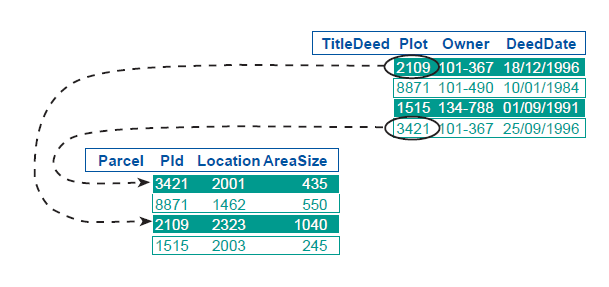
Figure 3: linking attributes to spatial entities (source: Huisman and de By, 2001)

3. GIS “third generation” - object model - e.g. Smallworld - storage of geometric and spatial data in a single database together as spatial objects - one of the ways to implement this strategy is eg object-oriented programming. This type of programming allows you to store, combine, search, manipulate and analyze information stored in a relational source without the need for a special database, without the need for any translation or data conversion, and without the need to store topology in a database in a special way. Spatial objects defined by an object-oriented database contain geometry as well as an attribute description. Permissible operations are defined for objects. Commands are executed by sending “messages” to all objects. Only those objects for which the given operation is allowed respond to these messages. Subobjects inherit behavior, but may have other properties. The model has no integrity problems (it is solved at the object level).
   
   

6.4 Query languages

The types of queries that the hierarchical and network database model allows are defined at the design stage of the database structure.

Written links in data records are used for browsing - orientation in the database. It follows that if we want to search the database, we must know the hierarchy in which the data is stored. Languages that require the user to know the database hierarchy are referred to as procedural query languages.

Relational databases achieve significantly greater flexibility by breaking down the hierarchy of attributes. Each attribute in them can be used as a key to search for information, and the data in separate tables can be related and associated using any attribute field that is common or that contains all the attributes. Unlike hierarchical and networked data structures, in relational structures, relationships are explicitly encoded in the database. Therefore, the relational model does not limit the scope of queries and the user does not need to know the structure of the database. The query language is thus not dependent on the data structure. We refer to such languages as non-procedural query languages. They are very popular and widespread. Probably the best known representative of this group of query languages is SQL (Standard Query Language) developed by IBM.

6.5 Geodatabase

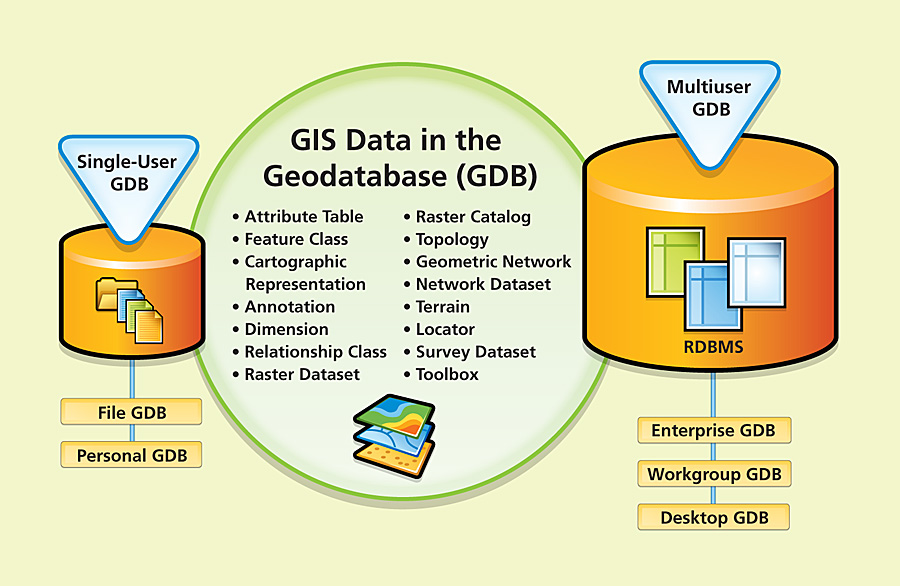
A geodatabase is a spatial database designed to store, query, and manipulate geographic information and spatial data. Geodatabase is a proprietary format developed by esri. This workspace manages both vector and raster data. The geodatabase is the natural data structure of ArcGIS and is the primary data format used for data editing and management.

The geodatabase repository model is based on a number of simple but necessary concepts of relational databases and uses the strengths of a basic database management system (DBMS). Simple tables and well-defined attribute types are used to store schema, rule, basis, and spatial attribute data for each geographic data set. This approach provides a formal model for storing and working with your data. With this approach, structured query language (SQL) — a number of relational functions and operators — can be used to create, modify, and query tables and their data elements.

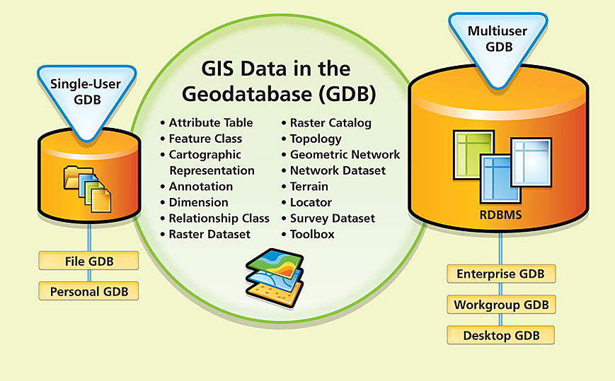
Figure 4: geodatabase concept (source:https://www.esri.com/news/arcnews/winter0809articles/winter0809gifs/p1p2-lg.jpg)

The geodatabase is implemented using the same multi-tier application architecture as in other advanced DBMS applications; there is nothing exotic or unusual about its implementation. The multilevel architecture of a geodatabase is sometimes referred to as an object-relational model. Geodatabase objects persist as rows in DBMS tables that have identities, and the behavior is delivered through the application logic of the geodatabase. Separating application logic from storage allows support for several different DBMS and data formats.

The key concept of a geodatabase is a dataset. The dataset is the primary mechanism for organizing and using geographic information in ArcGIS. We distinguish three basic types:

• Personal geodatabase - ArcGIS geodatabase data format stored and managed in Microsoft Access files (* .mdb). The entire contents of the geodatabase are stored in one MS Access file. This type of data storage limits the size of the geodatabase to 2GB. The effective limit before performance degradation is between 250 and 500 MB per MS Access file. For Microsoft Access experts and users, this is a good way to use a database with geographic data. The geodatabase contains tables with element classes and system tables containing information about advanced geodatabase options - subtypes, domains, sessions, etc. This type of geodatabase supports multiple readers and only one editor. One of the advantages of the geodatabase is the automatic calculation of geometric quantities - the length of line elements, the perimeter and the area of polygon elements. This is a dynamic value that updates when the element geometry changes.
• File geodatabase - this type of geodatabase is stored as a directory on the disk in the file system. Each dataset is maintained as a file that can be up to 1 TB in size. The 1 TB limit can be increased to 256 TB for extremely large raster datasets. Compared to a personal geodatabase, it reduces disk space by 50-75%. This type of geodatabase is preferred to personal geodatabases. It supports multiple readers and a single editor, but multiple editors for multiple datasets. The file geodatabase secures data in some way because it cannot be opened in a program other than ArcGIS. It also allows you to store data in a compressed, read-only format, which also reduces the space required for storage. Like the personal geodatabase, the file geodatabase is characterized by the automatic calculation of geometric quantities of individual elements, lines and polygons.
• ArcSDE geodatabase - geodatabase stored in a relational database using Oracle, Microsoft SQL Server, IBM DB2, IBM Informix or PostgresSQL. These multi-user geodatabases require ArcSDE to use and can run at unlimited sizes with an unlimited number of users. A set of different datasets that are maintained as tables in a relational database. The ArcSDE geodatabase supports reading and editing by multiple users. It is not a geodatabase freely and freely available in ArcGIS.

Size limits are based on DBMS limits.

6.5.1 Storing geodatabases in relational databases

The core of the geodatabase is a standard relational database schema (a series of standard database tables, column types, indexes, and other database objects). The schema persists in the collection of geodatabase system tables in the DBMS, which defines the integrity and behavior of geographic information. These tables are stored as files on disk or in DBMS content, such as Oracle, IBM DB2, PostgreSQL, IBM Informix, or Microsoft SQL Server.

Well-defined column types are used to store traditional table attributes. When a geodatabase is stored in a DBMS, spatial representations, most often represented by vectors or rasters, are generally stored using an extended spatial type.

Two primary sets of tables are stored in the geodatabase: system tables and dataset tables.

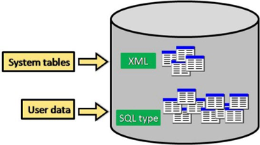
Figure 5: geodatabase table types

• dataset tables - each data file in the geodatabase is stored in one or more tables. Dataset tables work with system tables for data management.
• system tables - geodatabase system tables monitor the contents of each geodatabase. In essence, they describe a geodatabase schema that specifies all dataset definitions, rules, and relationships. These system tables contain and manage all the metadata needed to implement geodatabase properties, data validation rules, and behavior.

In the geodatabase, attributes are managed in tables based on a number of simple but necessary concepts of relational data:

• Tables contain rows.
• All rows in the table have the same columns.
• Each column has a data type, such as an integer, a decimal number, a character, and a date.
• There are a number of relational functions and operators (such as SQL) that work with tables and their data elements.

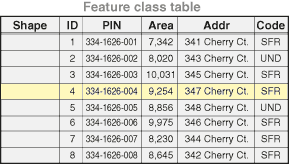
Figure 6: table structure

Tables and relationships play a key role in ArcGIS, as they do in traditional database applications. Rows in tables can be used to store all the properties of geographic objects. This includes holding and managing the geometry of an element in the Shape column.

Figure 7 shows two tables and how their records can be interconnected using a common field.

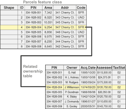
Figure 7: tables linking

6.5.1.1 Attribute data types in the geodatabase

There are several supported column types used to hold and manage attributes in the geodatabase. Available column types include various types of numbers, text, date, binary large objects (BLOBs), and globally unique identifiers (GUIDs). Supported attribute column types in the geodatabase include:

• Numbers: This can be one of four numeric data types: short integers, long integers, single-precision floating-point numbers (often referred to as floats), and double-precision floating-point numbers (commonly called doubling).
• Text: Any set of alphanumeric characters of a certain length.
• Date: Contains dates and time.
• BLOB: Binary large objects are used to store and manage binary information such as symbols and CAD geometry.
• Global Identifiers: The GlobalID and GUID data types store registry style strings consisting of 36 characters enclosed in curly braces. These strings uniquely identify a table element or row in the geodatabase and across geodatabases. These are very used to relationship management especially for data management, versioning, updating only changes and replication. Column types XML is also supported through programming interfaces. An XML column can contain any formatted XML content (such as XML metadata).

Extension tables

The tables provide descriptive information about elements, rasters, and traditional attribute tables in the geodatabase. Users perform many traditional table and relational operations using tables.

There is a targeted set of functions in the geodatabase that are optionally used to extend the capabilities of tables. These include the following:

• Attribute domains - specification of domains of individual attributes (setting of values that specific attributes can take) - suitable for ensuring the integrity of the database,
• Relationship classes - setting the relationship between two tables (linking, joining) using a common key - finds the rows of the second table in the given relation to the rows of the first table,
• subtypes - the organization of subclasses in a table - is often used when different subsets of one class of elements behave differently,
• Versioning - Manage long update transactions, historical archives, and multi-user modifications required in GIS workflows.

6.5.2 Feature Classes

Element classes are a homogeneous collection of common elements, each with the same spatial representation, such as points, lines, or polygons, and a common set of attribute columns, such as a class of line features to represent road centers. The four most commonly used function classes are points, lines, polygons, and annotations (the name of the geodatabase for map text).

Figure 4 shows the use of four datasets to represent the same area: (1) location of hatches as points, (2) sewer lines, (3) land polygons, and (4) annotation of street names.

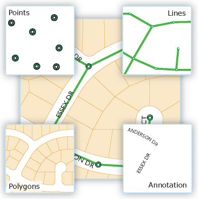
Figure 8: feature classes

Figure 8 shows the potential requirement to model some advanced feature properties. For example, sewer lines and manhole locations form a network of sewer networks, a system by which you can model runoff and flows. Also notice how the neighboring plots share common boundaries. Most package users want to maintain the integrity of shared function boundaries in their datasets using a topology.

As already mentioned, users often have to model such spatial relationships and behaviors in their geographic datasets. In these cases, you can extend these basic feature classes by adding a number of advanced geodatabase elements, such as topologies, network datasets, terrains, and address locators.

For more information about adding these advanced behaviors to geodatabases, see Feature Enhancements.

Types of feature classes

Vector elements (geographic objects with vector geometry) are universal and frequently used types of geographic data, suitable for representing elements with discrete boundaries, such as streets, states, and land. An object is an object that stores its geographical representation, which is usually a point, line, or polygon, as one of its properties (or fields) in a line. In ArcGIS, feature classes are a homogeneous collection of features with a common spatial representation and a set of attributes stored in a database table, such as a line feature class for representing road centers.

Note: When creating an element class, you will be prompted to set the element type to define the element class type (point, line, polygon, etc.).

In general, function classes are a thematic collection of points, lines, or polygons, but there are seven types of function classes. The first three are supported in databases and geodatabases. The last four are only supported in geodatabases:

• points = elements that are too small to represent as lines or polygons, as well as the location of points (such as GPS observations).
• lines - represent the shape and location of geographic features, such as street centers and streams, too narrow to be represented as areas. Lines are also used to represent elements that have a length but no surface, such as contours and borders.
• polygons - sets of multifaceted area elements that represent the shape and location of homogeneous element types, such as states, districts, lands, land types, and land use zones.
• annotation - Map text, including properties, as text is rendered. For example, in addition to the text string of each annotation, other properties are included, such as shape points for placing text, its font and point size, and other display properties. Annotations can also be linked to functions and can contain subclasses.
• dimension - a special type of annotation that shows specific lengths or distances, for example to indicate the length of the side of a building or the boundary of a plot or the distance between two elements. Dimensions are widely used in projects, engineering and GIS applications;
• multibody (multipoints) - consist of more than one point. Multipoints are often used to manage fields of very large point collections, such as groupings of lidar points, which can contain literally billions of points. It is not possible to use a single line for such point geometry. Grouping them into multipoint rows allows the geodatabase to process massive sets of points.