10 Geographical location, data preprocesing

10.1 From geoid to referrence elipsoid and sphere

From studying geography in primary and secondary schools, we have a rough idea of the shape of our planet Earth and its surroundings. In this chapter, we will introduce more detailed concepts describing its shape and how to determine its position on its surface. Although modern GIS tools allow for some forms of processing of three-dimensional reality, in our applications we will exclusively talk about a two-dimensional approach to space - that is, exclusively about describing the surface of the Earth.

The evolution of planet Earth has created a relatively rugged and rugged surface. We can imagine the simplicity of the mathematical description of the surface of a sphere or a rotating ellipsoid, from which the real shape of our planet is certainly very different. Every point of the Earth can be the subject of geodetic investigation. We therefore need some form of simplification that would lead to a universal mapping of the real surface of the Earth on the surface of a map (on paper).

A gradual simplification of the description of the shape of the Earth’s body is introduced. The initial approximation - actually a model - is the so-called geoid. We start from an idealized surface area of the Earth’s surface, which has been defined as the area where at each point on it the Earth’s gravity has the same value. We consider this surface to be at the level of the resting mean sea level (which is certainly not stable either). Thus it effectively extends below the land surface. In a sense, the surface of the geoid is the level of zero metres above sea level. The altitude figure itself is somehow debatable - the sea overflows in processes known as tides (tidal phenomena). Mean level is the average height between high and low tide (the difference in height in the Atlantic can be more than five metres). Elevation in Europe is usually related to the Baltic Sea.

Let us proceed to the definition of geoid:

Geoid is the zero level equipotential surface, which is at each point perpendicular to the direction of the earth’s gravity.

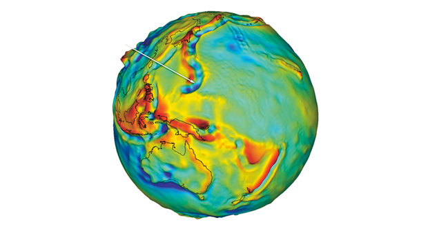
Figure 1: Geoid (source: https://www.abicko.cz/clanek/precti-si-technika-vesmir/22531/sisata-planeta-skutecna-podoba-zeme.html)

A typical geoid shape can be seen in Figure 2. The brown line shows the actual surface of the Earth, the blue line the area of the geoid and the black line the area of the surrogate ellipsoid. We can see that even the geoid is not easy to describe mathematically. In fact, it just smoothed out the wrinkled real topographic surface somewhat. Therefore, another model of the geoid is introduced and that is the surrogate ellipsoid. The replacement ellipsoid is already the beginning of cartography.

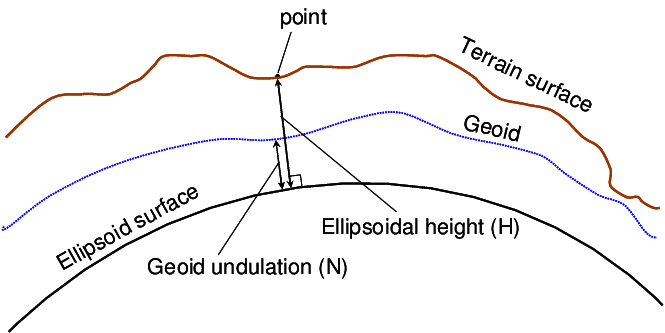
Figure 2: Geoid and Earth’s porosity (source: Ziebart et al., 2004)

Although the surface of the geoid is in some sense ideal, it is still difficult to describe mathematically. This is evident from the previous figure. Therefore, another approximation is introduced and that is the rotating ellipsoid. The rotational ellipsoid is a well-known geometric object that is given by its center and the lengths of the shorter and longer semi-axes. It is a so-called biaxial ellipsoid, which is formed by rotating the ellipse about the minor semi-axis. It can be expressed by the equation:

\(\frac{x^{2}+y^{2}}{a^{2}}+\frac{z^{2}}{b^{2}}=1\)

To clarify: in mathematical cartography, only the biaxial ellipsoid is used. There are two ways of approximating the Earth’s surface and related resulting ellipsoid types:

earth ellipsoid - created by approximating the geoid, the centre is identical to the centre of mass of the earth (geocentre), the minor axis is identical to the centre of rotation.
referential ellipsoid - formed by approximating a part of the geoid, the centre is not identical to the centre of the Earth, it approximates the selected area better than the Earth ellipsoid, representations defined on the rotational ellipsoid show less distortion than representations defined on the Earth ellipsoid.

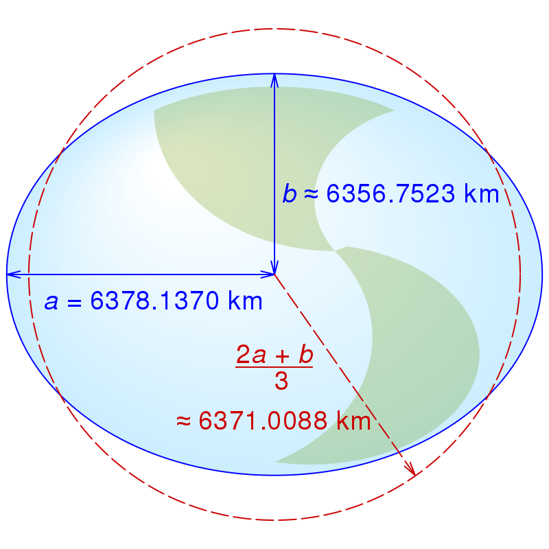
Figure 3: Reference ellipsoid (source: https://cs.wikipedia.org/wiki/Referenční_elipsoid)

Thus, in GIS related fields, the rotating ellipsoid is most commonly called reference (surrogate) ellipsoid. This ellipsoid can be specified in different ways - choosing the length parameters of the shorter and longer axes. Different choices of ellipsoid replace the geoid with different accuracy (truthfulness), because the ellipsoid fits differently at different places on the geoid (the distance of the geoid surface from the ellipsoid changes). The choice of an alternative ellipsoid is therefore a matter of compromise, usually valid only for smaller areas (national ellipsoids). The choice of an alternative ellipsoid for a particular application is called in the English literature date.

For the purposes of larger mapping works, it is necessary to relate the data to a global ellipsoid that would cover the entire planet. The global ellipsoid has evolved over a long period of time and was not settled until 1984 in a form called WGS-84. However, its use is inappropriate for national geodesy purposes. The parameters of the best known ellipsoids are shown in Figure 4.

Figure 4: The most famous ellipsoids (source: https://web.natur.cuni.cz/~bayertom/images/courses/mmk/mk0.pdf)

The reference ellipsoid can then be replaced by a simpler solid, namely a reference sphere, which has a simpler mathematical definition. The reference sphere has larger deviations from the geoid than the ellipsoid. Its radius \(R\) can be chosen in various ways and has the following properties:

constant curvature,
it is easier to perform calculations on,
it is suitable for small and medium scale maps (not state map work).

The reference sphere (Figure 5) can be replaced:

ellipsoid locally (area 300 x 300 km) - precise calculations on a small area (differences can be neglected),
ellipsoid globally - less accurate calculations over the entire surface of the Earth - use in geographic cartography.

Cartographic distortions when replacing a geoid with a sphere are 2 orders of magnitude (100x) greater than when replacing a geoid with an ellipsoid.

Figure 5: Reference sphere and reference ellipsoid (source: http://gisak.vsb.cz/GISacek/GISacek_2001/sbornik/Hanzlova/Hanzlova.htm)

When replacing an ellipsoid by a sphere on a small area, we can choose its radius \(R\) in the following ways:

\(R=a\),
\(R=b\),
\(R\) is the mean radius of curvature \(R=\sqrt{MN}\). nzlova.htm)](./pictures/reference_balls.png)

Replacing the ellipsoid globally can be done in the following ways:

The sphere will have the same volume as the ellipsoid, \(R=\sqrt[3]{a^{2}b}\);
The sphere will have the same surface as the ellipsoid, \(R=b^sqrt{(1+\frac{2}{3}e^{2}+\frac{3}{5}e^{4}+\frac{4}{7}e^{6}\dots)}\);
The diameter of the sphere is expressed as the arithmetic mean of the semi-axes: \(R=\frac{2a+b}{3}\).

When creating a two-dimensional map, it is then necessary to convert the image from a three-dimensional template (reference ellipsoid or reference sphere) into a plane. The surface on which we display objects from the reference surface is called the display surface. The most commonly used surfaces developed into a plane are the conic, cylindrical, or tangent plane. It is possible to display on more than one surface (polyconic displays).

10.2 Geographical location

Before we can work with geofeatures, we need to clearly define their position in space. For this purpose, we can use a number of different so-called spatial reference systems (Figure 6), describing the position of geofigures in different ways, with different accuracy and resolution.

Figure 6: Spatial reference systems (source: Rapant, 2002)

There are basically two ways to determine the position:

directly using coordinate systems (georeferencing),
indirectly using geocodes (geocoding). <(geoinformation) can be used by means of geoinformation (e.g. by using georeferencing).

10.2.1 Direct positioning (georeferencing)

In the case of direct positioning using coordinate systems, we distinguish:

global coordinate systems,
local coordinate systems.

10.2.1.1 Global coordinate systems

Global coordinate systems are those that are used for positioning within large areas (the whole Earth, a country or at least a large part of a country). In terms of positioning continuity, global coordinate systems are divided into:

continuous coordinate systems,
discrete coordinate systems.

Global continuous coordinate systems

Continuous coordinate systems are based on the continuous measurement of the position of geoelements, without step changes in coordinates and interruptions. They can be subdivided according to the method of deriving the position of the geofeatures into:

absolute,
relative.

Since relative positioning is practically not used in the case of global systems, we will only discuss the absolute variation, where the position is given directly by the coordinates expressed in the global coordinate system.

These coordinate systems can be defined in relation to:

the earth’s body,
the plane on which the earth’s surface is projected.
absolute,
relative.

Figure 7: Geographic coordinate system (source: http://tvorbamap.shocart.cz/kartografie/projekce.htm)

There are usually two basic coordinate systems related to the earth’s body:

geographic coordinate system (spherical in principle) - the position of a point on the Earth’s surface (Figure 7) is given by latitude \(\varphi\) and longitude \(\lambda\). Longitude is given in degrees, with zero degrees corresponding to the Greenwich (zero) meridian. Latitude is also given in degrees, zero degrees corresponds to the equator, \(90^{o}\) corresponds to the poles. Geographic coordinates are sometimes supplemented by the altitude \(h\), given in metres. The * Cartesian coordinate system, starting at the centre of the Earth (Figure 8), gives the position of a point using a triplet of coordinates \([x,y,z]\). The \(x\) and \(y\) axes lie in the plane of the equator, the \(x\) axis passes through the intersection of the zero meridian and the equator, the \(z\) axis is perpendicular to them and usually identical to the Earth’s axis of rotation.

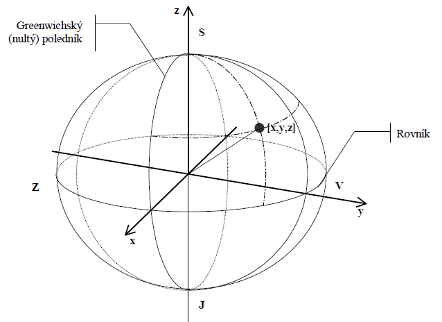
Figure 8: Cartesian coordinate system (source: Rapant, 2002)

The essential difference between these two systems is that while in the case of the geographic coordinate system the position is defined by only two coordinates and it is automatically assumed that the described point lies on the surface of the Earth, in the case of the Cartesian coordinate system the position is described by three coordinates. The advantage of the Cartesian coordinate system is that it can be used to describe the position of any point, even above or below the surface of the Earth.

Coordinate systems related to the plane on which the Earth’s surface is projected

The coordinate systems belonging to this group are numerous and are related to cartographic techniques, i.e. the representation of the Earth’s surface on maps. If we want to represent a large part of the Earth’s surface (where curvature can no longer be neglected) on a flat map, we have to perform the following transformations:

reducing the scale so that the area to be depicted fits on a sheet of paper of the desired size,
project the curved surface onto the plane in a systematic way. This projection is called cartographic mapping and is essentially a systematic transformation of the geographic coordinates \((\varphi,\lambda)\) into the corresponding planar coordinates \((x,y)\) of the map. Mathematically, this transformation can be written as follows:

\(x=f_{1}(\varphi,\lambda)\)

\(y=f_{2}(\varphi,\lambda)\)

a schematicky naznačit

\((\varphi,\lambda)\longrightarrow (x,y)\)

This transformation usually consists of several steps (as mentioned above):

Transformation of the Earth’s surface into a geoid surface. The surface of the globe is too rugged to work with effectively. Therefore, the Earth’s surface is usually replaced by a surrogate surface that adheres as closely as possible to the actual terrain, but does not take into account irrelevant details, the omission of which will not significantly affect the quality of the resulting work.
Transformation of a geoid surface into a biaxial ellipsoid surface. Since the geoid is a very general surface, it is necessary to replace it with another surface that is mathematically easy to describe and thus easy to work with. For this purpose, the rotating biaxial ellipsoid has proved to be the most suitable. Over time, cartographers have introduced a variety of ellipsoids suitable for different purposes and for representing different parts of the Earth’s surface (Figure 4). The reference ellipsoid is used in the definition of national and international geodetic coordinate systems, and in the production of large and medium scale map works where minimal distortion is required.
Transformation of the surface of the ellipsoid to the surface of the sphere. The reference ellipsoid is replaced by a reference sphere. Sometimes the reference sphere is used instead of the rotating ellipsoid. This is the case when we have lower demands on the accuracy of the representation, e.g. in the case of creating small scale maps, e.g. wall or atlas maps.
Transformation of the surface of a sphere into a surface developable into a plane (cylinder shell, cone shell, tangent plane).
Developing the surface into a plane and introducing a rectangular coordinate system.

There is a wide range of cartographic displays available today. For example, in the Czech Republic, the Křovákovo cartographic representation (and its corresponding S-JTSK coordinate system) is commonly used, which was created specifically for the former Czechoslovak Republic and which respected its elongated shape and position on the globe.

The Government of the Czech Republic issued Decree No. 430/2006 Coll. on the determination of geodetic reference systems and state map works binding on the territory of the state and the principles of their use, which established binding geodetic reference systems for the territory of our state:

World Geodetic Reference System 1984 (WGS84),
European Terrestrial Reference System (ETRS),
Coordinate system of the Unified Trigonometric Cadastral Network (S-JTSK),
Gusterberg Cadastral Coordinate System,
St. Stephen’s Catastral Coordinate System,
Baltic height system - after levelling (Bpv),
Gravity system 1995 (S-Gr95),
Coordinate system 1942 (S-42/83).

The parameters of these geodetic reference systems are also listed in the Annex to this Regulation.

Global discrete coordinate systems

Global discrete coordinate systems also exist practically only in the absolute version. They can be defined again in relation to:

the earth’s body,
the plane onto which the earth’s surface is projected.

An example of a global discrete coordinate system related to the earth’s body may be the spherical grid (Figure 9), which covers the surface of the globe. It is derived from an octahedron inscribed in the globe, whose triangular faces are successively divided into smaller and smaller triangles, with the newly generated vertices being adjacent to the surface of the globe (Figures 10 and 11).

Figure 9: Spherical grid - basic octahedron (source: Rapant, 2002)

!Figure 10: Spherical grid - sample result after the fourth division (source: Rapant, 2002)](./pictures/spherically_grid1.png)

!Figure 11: Spherical grid - sample of division and addressing (source: Rapant, 2002)](./pictures/spherically_grid2.png)

Coordinate systems related to the plane on which the Earth’s surface is projected

These coordinate systems are used almost exclusively when working with raster data. It is typical for them that the coordinates are changed by a jump. The position is defined by regularly spaced planar elements, usually square in shape, corresponding to individual cells. Within the grid, a local coordinate system is usually used, with the origin usually in the upper left corner of the grid, the \(x\)-axis going in the left-to-right direction and the \(y\)-axis going in the top-to-bottom direction (Figure 12).

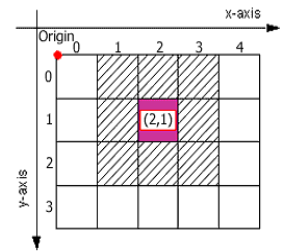
Figure 12: Discrete coordinate system (source: https://www.esri.com/about/newsroom/arcuser/understanding-raster-georeferencing/)

However, in practical work with rasters in a GIS environment, we usually do not work with local discrete coordinates, but usually transform them into a global continuous coordinate system. It is then possible to determine the global coordinates of individual cells. In doing so, it should be assumed that the coordinates are always the same (constant) for the whole cell area, corresponding either to the global coordinates of one of the cell corners or to the cell center. The coordinates change by a jump when the boundary between two cells is crossed.

10.2.1.2 Local coordinate systems

These coordinate systems are again divided according to the smoothness of the coordinate change into:

continuous coordinate systems,
discrete coordinate systems.

Local continuous coordinate systems

Local continuous coordinate systems are based on continuous measurement of the position of geo elements, without step changes in coordinates and interruptions.

They can be further divided into:

absolute,
relative.

Absolute coordinate systems are based on positioning using coordinates indicating distance along coordinate axes relative to a common origin.

Relative systems, on the other hand, are based on the positioning of geofeatures using coordinates indicating the distance along two specified directions from an origin that is identified with a known, fixed and easily recognizable point in the terrain (e.g., a corner of a house, an entrance to a house, etc.).
>

Absolute local continuous coordinate systems

These coordinate systems can practically only relate to the plane. They are essentially represented by a local coordinate system (in the narrower sense), which is defined by a randomly chosen origin and two directions of the coordinate axes and which is valid only in a limited area. The use of such systems has advantages and disadvantages. The main advantage is that we can measure practically anywhere and at any time, we are not dependent on the design of the so-called coupling device by which we connect to the global coordinate system (e.g. S-JSTK).

The disadvantage, however, is that it is usually only a matter of time before this local system needs to be linked to the global system. And then there is usually nothing to do but to re-aim a few points, this time in absolute coordinates, and then transform the local system into the global one, or do the whole measurement again.

Relative local continuous coordinate systems

These coordinate systems can be defined in relation to:

plane - these are relative systems indicating position relative to certain fixed localised objects whose position is also known in absolute coordinates. In essence, it is a modification of the previous case, with the origin of the local coordinate being the origin of the local coordinate. The origin of the system is identical to a prominent point on the terrain surface (e.g. a corner of the house, an entrance or a point marked in a special way on the wall of the house) and the directions and orientations of the axes are also given in relation to prominent directions on the terrain surface (e.g. along and perpendicular to the wall of the house). Such coordinate systems are commonly used to locate the course of lines and control elements of utility networks, e.g. water and gas pipes (the well-known plates on the facades of houses), or underground high-voltage electric cables. The disadvantages of these systems are usually an incomplete description of the course of the lines, low accuracy and difficult transformation into global coordinates, resulting also from the fact that practically for each localised point a new local coordinate system is always introduced. Disadvantages also include the fact that different utility managers relate the location of their lines to different landmarks and their maps are then difficult to compare, if comparison can be made at all. Disadvantages also include the possibility that the original landmark may be destroyed (e.g. due to demolition of a house) and thus the loss of ‘orientation’.
lines - dynamic segmentation - coordinate system used for determining the relative position of geoelements with respect to the starting point (“origin”) along a given line (called stationing). This coordinate system (Figure 13) is very often used by managers of transport networks (roads, railways, watercourses). For example, along railways, bollards are placed with the distance from the origin of the line. In the case of railways, the use of such a coordinate system is probably the least problematic. After all, lines are not so often translated. However, the situation is far worse in the case of the road network and watercourses, especially in the context of the transition to the use of GIS. In principle, two sources of difficulty can be distinguished here:
- problematic periodic updating of geo-fragment coordinates - when adjusting the course of roads and watercourses, the relative position of all geo-fragments relative to the origin is usually not measured,
- generalization of line features in the GIS environment - generalization generally leads to shortening of lines, i.e. if in this situation we start to enter the position of geofences (canals, parking lots, utility closures, etc.) along the road image in the GIS according to the originally recorded distances, the geofences will gradually start to move away from the origin along the line compared to the actual position.

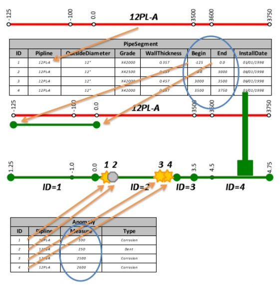
Figure 13: Example of stationing in a pipe network

Both problems can be largely avoided by, for example, building a system of “bollards” along a given line, which indicate precisely defined distances from the origin of the line (e.g. river kilometres), and then determining the position of the geofences by measuring from these “bollards”. This creates a system of local coordinate systems, always valid in the area between two ‘bollards’. This results in a situation where positioning errors along the line are not added up over the entire length of the line, but only within the intervals between the ‘footers’. However, two conditions must necessarily be met:

to have all the bollards accurately located, and to update their position in case of modifications;
the actual representation of the line (road, watercourse) in the map must necessarily pass through these “footers”.
>

How to do it in ArcGIS? Watch the videos:

Local discrete coordinate systems

Again, these coordinate systems exist only in absolute form and refer to the plane. Basically, these coordinate systems are used exclusively when working with raster data. It is typical for them that the coordinates change by a jump. The position is defined by regularly spaced planar elements, usually square in shape, corresponding to individual cells. Within the raster, a local coordinate system is usually used, with the origin usually located in the upper left corner of the raster, the i-axis going in the left-to-right direction and the j-axis going in the top-to-bottom direction (Figure 12). The cell dimensions are taken as unit. Transformation to the global coordinate system is not introduced in this case.

Recommended resources for further study:

Richard Knippers: Geometric Aspects of Mapping

10.3 Data preprocessing

There are different classifications of GIS project activities, but most of them recognize a stage where digital data is manipulated, but the purpose of this manipulation is not to perform analyses, syntheses or produce outputs. This stage is often referred to as ‘data preprocessing’, ‘restructuring, generalisation and transformation’. Opinions on the classification of specific activities in this stage are also not uniform.

One of the basic forms of data manipulation is selective spatial editing of geometric objects while changing topological relationships. Many vector GISs have the capability to perform data modifications at certain limited locations in the database. This operation is called partial processing, or partial processing (e.g., adding a line to divide an existing surface into two changes topological relationships).

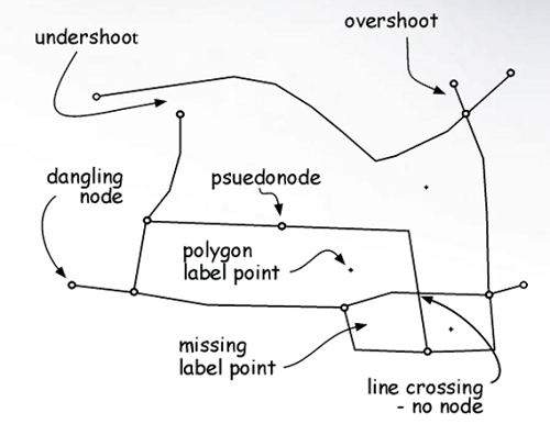
Obrázek 14: Topologické chyby vzniklé při digitalizaci (zdroj: is.humboldt.edu/OLM_2016/Lessons/GIS/08 Rasters/Images/)

Data preprocessing represents activities aimed at processing the acquired data into the desired form. It will not be a process in terms of data analysis and synthesis, but rather a preprocessing of the data for these procedures. The whole process of data processing (preprocessing) can be divided into sub-steps: data restructuring, geometric transformation of representations and map projection change, data conversion and image processing, generalization.

10.3.1 Data Restructuring

Restructuring of data means intervention in all parts of geo-data in order to adapt them for further processing, e.g. change of topological relations, spatial distribution of vector and raster representations, identification of edges, change of resolution, manipulation of attribute values.

In GIS systems it is necessary to organize a large volume of spatial data in a database, therefore different methods of spatial partitioning of vector representations are used. The most common is the division according to a predefined square grid or a set of regular boundaries that define the individual parts - “map sheets” - sheets or tiles. This process is often referred to as tiling. However, the territory contained in a geographic database may also be divided into irregular sheets. This division is more flexible, but requires more complex processing. It is mainly used when we follow the division of territories according to national, regional or other boundaries.

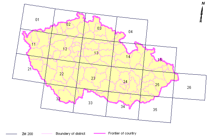
Figure 15: Territorial division - ZM 1:200 000 sheet cladding (source: http://zpravodajstvi.ecn.cz/rtk/catalogue-gis/eng/polohop/arccr/klad.htm)

!Figure 16: Splitting satellite image into tiles (source: http://www.avenza.com/help/geographic-imager/5.0/tiling_images.htm)](./pictures/tile_example.png)

The spatial division of the database into parts (map sheets) requires careful management of the edges of individual sheets. Edge-matching is a process that ensures the joining of separated (map) sheets into a continuous map and at the same time the linking of objects that extend into both joined sheets. In this process it is necessary to rebuild the topology of the objects that interfere with both joined sheets.

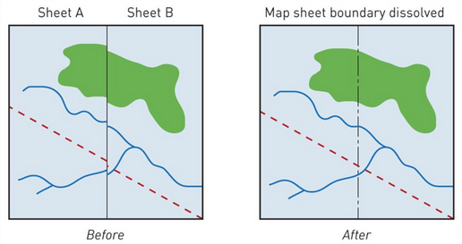
Figure 17: Edge matching (source: http://www.avenza.com/help/geographic-imager/5.0/tiling_images.htm)

10.3.2 Geometric transformation of representations and change of the projection

Geometric transformation involves the process of converting geographic coordinates to rectangular plane coordinates, called analytic transformation, and converting coordinates between rectangular plane coordinates, called Numeric transformation. The transformation mechanisms are based on the transition defining the position of the corresponding reference ellipsoid. GIS systems offer powerful means for performing analytical transformations of various kinds. Changes between them are performed by means of the definition of a position on the corresponding ellipsoid. Such changes are usually referred to as projections.

When working with GIS, we often work with three cartographic views:

the input map view,
the internal view of the system,
the map output view.

Often, the input map data are made in different cartographic representations and scales, so it is necessary to transform them into an internal unified coordinate system. Coordinate transformations between planar rectangular coordinate systems are called numerical transformations. They do not require knowledge of the mapping equations of cartographic transformations to the original and new coordinate system. They are based on knowing the exact position of the selected points in both coordinate systems. In practical applications, two methods are used:

linear conformal transformation (Helmert) - is given by relations:

\(x´=m\cdot x\cdot \cos \beta+m\cdot y\cdot \sin \beta+a\)

\(y´=-m\cdot x\cdot \sin \beta+m\cdot y\cdot \cos \beta+b\)

is suitable for transformation between coordinate systems that are offset, rotated and scaled in the same ratio in the directions of both coordinate axes. The transformation parameters are determined by reference points whose coordinates are known in both coordinate systems. In order to estimate the transformation parameters optimally, a larger number of reference points are used. The values of the transformation coefficients are then calculated using the least squares method, which minimizes the sum of the position differences between the coordinates of the reference points in the two coordinate systems.

polynomial transformation - its special case is the affine transformation (first order polynomial transformation), which is given by relations:

\(x´=a\cdot x+b\cdot y+c\)

\(y´=d\cdot x+e\cdot y+f\)

The coefficients of the transformation equations are also calculated using the least squares method. The affine transformation is used when transforming the digitizer coordinate system to the map coordinate system.

For raster representations, the process of resampling of cell data is of the nature of analytical and polynomial transformations. During resampling, the position of the centre of each cell of the new representation in the coordinate system of the input representation is calculated according to the transformation equations - it is transformed into it. After identifying the cell center, it is possible to assign or calculate an attribute value for it from the values stored in the cells of the original representation. There are several techniques to determine this attribute value:

nearest neighbour assignment - the transformed position of the cell center is assigned the attribute value stored in the cell of the original grid whose center is located closest to the transformed one

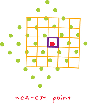
Figure 18: resampling by nearest neighbor method (source: https://support.esri.com/en/other-resources/gis-dictionary)

bilinear interpolation - the centres of the four closest cells of the original representation to the transformed centre of the output cell are identified and the average value of these four cells is assigned, weighted by the distance

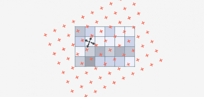
Figure 19: Resampling by bilinear interpolation (source: https://gisgeography.com/bilinear-interpolation-resampling/)

cubic convolution - similar to bilinear interpolation, but the assigned value is calculated as a distance-weighted average of the sixteen nearest values of the input representation

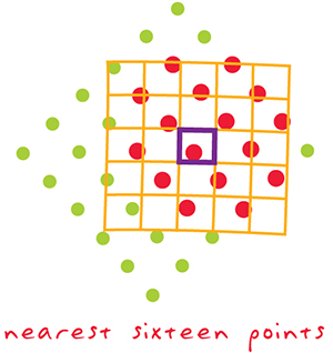
Figure 20: resampling by the cubic convolution method (source: https://support.esri.com/en/other-resources/gis-dictionary)

10.3.3 Převod dat a zpracování obrazu

Image processing is a process that is mainly used for raster systems and remote sensing. In GIS, the use is limited; therefore, the following list of documents contains only a fraction of the functions that this process encompasses. Image processing functions include: filtering (edge detection, smoothing and sharpening of boundaries), histogram modification, brightness and contrast modification, classification, etc. Data conversion allows the transition between vector and raster data formats. During rasterization (vector to raster format conversion), the vector layer is overlaid with a raster grid of cells of fixed size to which the correct attribute is assigned. Problems with this conversion can occur when one cell contains parts of multiple objects after overlay. The resulting situation is then handled by the centroid method, the dominant type method, or the most important category method. The vectorization of points is relatively simple. In the vector representation, the location of the point corresponding to the center of the raster cell is identified. Similarly, it is possible to proceed with lines when adjacent cells are connected.

10.3.4 Generalization

Generalization in a GIS environment is a process that aims to generalize the contents of a spatial database for map display and communication processes and analytical processes. The first requirements for generalisation are economic requirements, which emphasise that any modelling of reality requires financial resources and is also constrained by technical developments. Next in line are data reduction requirements that combine generalization with the need to filter out potential errors arising in the GIS creation process. The final reason for generalisation - the requirement for visualisation and perception of the data - is based on basic cartographic recommendations that (with respect to map legibility) indicate the degree of fulfilment. The most common generalization techniques are: selection - selecting elements, elimination - removing elements, simplification of elements, aggregation - combining smaller elements into larger ones, spatial reduction of elements, typification - reducing the density of elements, exaggeration - highlighting elements , reclassification and linking elements, conflict resolution, refinement - smoothing elements or reducing peaks.

When generalizing vector data, the emphasis is on simplifying and improving the representation of linear objects. Their quality evaluation is based primarily on the requirement of preserving the information structure. A purely geometric approach to generalization is often criticized, so in practice, combined approaches are often used. The simplest approach is to keep only some of the line breakpoints according to a systematic selection. However, this procedure does not ensure perfect preservation of the line shape. Another option is to remove points that are too close to their neighbours or have too small a difference angle between vectors. In this procedure, a mask containing three points (vertexes) from the origin to the end point of the line can be used. These vertexes are evaluated in terms of the distance and difference angle of the straight line segments. If the difference angle or distance is less than a specified limit, the point is removed.