12 Raster data analysis

One of the previous chapter described some of the commonest data structures for the storage of raster data and emphasized that at least one of the reasons that they were developed was to produce smaller files for raster GIS layers. Smaller files mean that less disk space is needed to store them and that it will be quicker to transfer them between the disk and the memory of the computer. A small file size should also mean that operations on the layers, such as queries and overlays, should run more quickly, because there is less data to process. However, this will only be true if the query can use the raster layer in its compressed form, whether this be run length encoded or in a quadtree or in any other format. If this is not possible then the layer would haVe to be conVerted back to its original array format (which would take time) and then the query run on this expanded form of the data. So the data structures which are used for raster data not only haVe to produce savings in file size, they must be capable of being used for a range of GIS queries.

Raster analyses range from the simple to the complex, largely due to the early inven- tion, simplicity, and flexibility of the raster data model. Rasters are based on two- dimensional arrays, data structures sup- ported by many of the earliest programming languages. The raster row and column for- mat is among the easiest to specify in com- puter code and is easily understood, thereby encouraging modification, experimentation, and the creation of new raster operations. Raster cells can store nominal, ordinal, or interval/ratio data, so a wide range of vari- ables may be represented. Complex con- structs may be built from raster data, including networks of connected cells, or groups of cells to form areas.

The flexibility of raster analyses has been amply demonstrated by the wide range of problems they have helped solve. Raster analyses are routinely used to predict the fate of pollutants in the atmosphere, the spread of disease, animal migration, and crop yields. Time varying and wide area phenomena are often analyzed using raster data, particularly when remotely sensed inputs are available. The long history of raster analyses has resulted in a set of tools that should be understood by every GIS user. Many of these tools have a common conceptual basis and they may be adapted to several types of problems. In addition, specialized raster analysis methods have been developed for less frequently encountered problems. The GIS user may more effectively apply raster data analysis if she understands the underly- ing concepts and has become acquainted with a range of raster analysis methods.

12.1 Raster algorithms: attribute query for run length encoded data

The first is the most basic query of all - reporting the Value in a single piXel. To illustrate this we will use the simple layer in Figure 1, and imagine that we wish to find out the attribute Value stored in the piXel in row 2 column 3. Remember that rows and columns are numbered from zero.

In a real GIS of course, this query is more likely to take the form of an on-screen query, in which the user clicks a graphics cursor oVer the required piXel on a map produced from the data. HoweVer, it is a simple matter for the software to translate the position of the cursor to a piXel position on the layer itself.

Figure 1: Example of simple raster array (source: Wise, 2002)

We haVe already seen how this query would be answered using the array data structure. Assuming the layer is stored in an array called IMAGE, the Value we want will be held in the array element IMAGE[2,3]. To retrieVe this Value from the array as it is stored in memory (Figure 2) we calculate the address from the row and column number by first calculating the offset - how many elements along the array we need to go:

$offset = (nrow*rowsize)+ncolumn$ $offset = (2*4)+3=11$

Figure 2: Storage of array in computer memory (source: Wise, 2002)

To find the actual address in memory, we add the offset to the address of the first element, which is 200

$address = origin + offset = 200+11=211$

If we look at Figure 2, we can see that the Value in address 211 is B, which is correct.

Notice that the addresses are different from those giVen in Chapter 6. This is deliberate because the actual addresses will normally be different eVery time the software is run. When a program, such as a GIS, is loaded into memory ready to be run, where eXactly in memory it goes will depend on what is already running on the computer. If this is the first package to be run, then it will be loaded near the start of the memory (and the addresses will be small numbers). If there are already other programs running, such as a word processor or spreadsheet package, then the GIS will go higher in memory and the addresses will be larger numbers. One of the things which happens when a program is loaded into memory, is that the origins of all the arrays are discovered and stored, so that all the array referencing in the program will work properly.

If we look at the same raster layer stored in run length encoded form (Figure 3), we can see that this same approach is not going to work because there is no longer a simple relationship between the addresses and the original row and column numbers. For instance, the Value stored at offset 4 will always refer to the second run found in the original layer but which row and column this relates to depends entirely on the length of the first run. What we have to do is work out the offset ourselves, and then count along the runs until we find the one that contains the pixel we want.

Figure 3: Storage image in run length encoded form in computer memory (source: Wise, 2002)

The Run length Encoded storage of the image is declared as a one-dimensional array on line 1. Since we cannot take advantage of the automatic facilities provided by the 2D row and column notation, we may as well treat the image in the way that it is actually stored in memory - as a single row of Values. Line 2 calculates the offset, and is the same as the calculation that is done automatically when the image is stored using a 2D array. The key to this algorithm is line 6. The first time through this program, both pos and n will haVe the Value 0 (set on lines 3 and 4). RLE[O] contains the length of the first run (3) so pos will take the Value 3. If this is greater than or equal to the offset we are looking for (line 8), then this first run would contain the piXel we are looking for. HoweVer it does not, so we go back to the start of the repeat loop on line 5. When line 6 is eXecuted this time, n has been set to a Value of 2 (on line 7) so RLE[2] will giVe the length of the second run - 1. This is added to pos, making 4, which is still less than our offset, so we go round the repeat loop again.

Eventually, on the sixth time around, the Value of pos will reach 12 - this means we haVe found the run we are looking for and the repeat loop ends. By this stage, n has a Value of 4, since it is pointing to the length of the next run, so we look at the Value in the previous array element to get the answer - B. It is immediately clear that this algorithm is less efficient than the one for the array. In fact, every time we make a reference to an element in RLE in this example, the computer will haVe to do the same amount of work as it did to retrieve the correct answer when we stored the data in an array. Answering this query using an array had order O(1) time efficiency - it works equally quickly, no matter how large the raster layer. In the case of the run length encoded data structure, the time taken is related to the number of runs which are stored. Other things being equal, we might expect this to be related to the size of the layer. The layer is 4 4 pixels. If we doubled the size to 8 8, the number of pixels would go up by a factor of 4. However, the number of runs would not go up quite this much, because some runs would simply become longer. The exact relationship would depend on how homogeneous the pattern of Values was. A reasonable assumption is that the runs would roughly double in size if n doubled - hence our algorithm would have O(n) processing efficiency.

12.2 Raster algorithms: attribute query for quadtrees

We seem to face the same problem in carrying out our attribute query using a quadtree as we did with the run length encoded Version of the layer - there appears to be no relationship between the position of the pixels in the original GIS layer, and their position in the data structure (Figure 5). HoweVer, oddly enough, this is not the case, because when we created the quadtree, we saw that we were able to give each ‘pixel’ in the tree a Morton address (shown on Figure 4), and there is a relationship between these Morton addresses and the row and column numbers.

Figure 4: Quadtree subdivision of layer with the piXel in column 3, row 2 highlighted. (source: Wise, 2002)

Let us take the same query as before - find the Value of the pixel in column 3, row 2. To discoVer the Morton address we first haVe to convert the column and row to binary. For those who are not familiar with changing between number bases, this is explained in detail in a separate box - those who are familiar will know that the result is as follows:

$3_{10}=11_2$ $2_{10}=10_2$

where the subscript denotes the base of the numbers. We now have two, 2-bit numbers - 11, and 10. We produce a single number from these by a process called interleaving. We take the first (leftmost) bit of the first number followed by the first bit of the second number, then the second bit of the first number and the second bit of the second number as shown below:

First bit of 11	First bit of 10	Second bit of 11	Second bit of 10
1	1	1	0

This produces a new number 11102. Finally, we convert this from base 2 to base 4 which giVes 324. Again this is explained separately in the box for those who are unfamiliar with conversion between different number bases. If you look at Figure 4, you can see that this is indeed the Morton address for the pixel in column 3, row 2. So why does this apparently odd process produce the right answer? The answer lies in the way that the Morton addresses were derived in the first place.

One of the problems with spatial data is just that - that they are spatial. One of the most important things to be able to do with any kind of data is to put it into a logical sequence, because it makes it easier to find particular items. We have already seen how haVing a list of names in alphabetical order makes it possible to find a particular name using things like a binary search. This algorithm is only possible because the names are in a sequence. But how can we do the same with spatial data, which is 2D?

If we take pixels and order them by their row number, then pixels which are actually Very close in space (such as row 0, column 0 and row 1, column 0) will not be close in our ordered list. If we use the column number instead we will haVe the same difficulty. This was the problem that faced the deVelopers of the Canadian GIS, and the solution they came up with was to combine the row and column numbers into a single value in such a way that pixels that were close in space, were also close when ordered by this Value. The Morton code, named after its inVentor, was the result. Therefore, the reason that quadtree pixels are labelled in this way is because there is then a simple means of deriVing their quadtree address from the row and column number. The Morton code is also known as a Peano key, and is just one of a number of ways in which pixels can be ordered. The question of how spatial data can be organized to make it easy to search for particular items is a Very important one, and will be considered further.

Figure 5: Storage of quadtree in memory. (source: Wise, 2002)

Let us return to our original query. The next stage is to use our Morton address of 31 to retrieve the correct value from the data structure in Figure 5. Each digit in the Morton address actually refers to the quadrant the pixel was in at each leVel of subdiVision of the original layer, and this is the key to using the address in conjunction with the data structure. In this case, the first digit is 3, which means the piXel was in quadrant 3 when the layer was first subdivided (this can be checked by looking at Figure 4). When we stored the quadtree in our data structure, the results for the first subdivision were stored in the first four locations, starting at offset 0. (Note that to simplify this eXplanation, the storage elements in Figure 5 are shown in terms of an offset, rather than a full address in memory as was done for the example of run length encoding). The value for piXel 3 will therefore be stored in offset 3 - the first digit of the Morton address points directly to the location we need. The value stored in offset 3 is number 12. Since this is a number, rather than a letter, it means that the results of the second subdivision are stored in the four locations starting at offset 12. The second digit of our Morton address is a 2, so the value we are looking for will be stored in the location which is offset from 12 by 2 - a new offset value of 14. Looking at Figure 7.5, we can see that the value stored at offset 14 is indeed B, the answer to our query.

What would haVe happened if we had requested the value for the piXel on row 0, column 1? The Morton address in this case would be 00012, or 014. Note that we do not leave off the leading zeroes from these addresses. Applying the same algorithm as before, we take the first digit, 0 and look in our data structure. This time we find a letter, A, rather than a number. This means that we have found a leaf, rather than a branch, and in fact this is the answer to our query. There is no need to use the other digits in the Morton address, since all the pixels in quadrant 0 at the first subdivision had the same value.

As with the run length encoded version, we treat the quadtree as a single array, and find our way to the correct element of the array using an algorithm rather than the in-built system which we had with the 2D array. In our simple example, we had a 4x4 image, which was diVided into quadrants two times. If we doubled the size of the image to 8 8, this would only add one to the number of subdivisions, which would become 3. You will probably haVe noticed a pattern here, since

$4=2^2$ $8=2^3$.

In other words, the maXimum number of levels in a quadtree is the number of times we can divide the size of the quadtree side, n, by 2 - in other words $\log_2 n$. This means our algorithm for finding any giVen pixel has processing efficiency which is $O(\log n)$.

Before we leave this particular algorithm, it is worth taking time to explore the fourth line in the code sequence above since it affords a useful insight into the way that computers actually perform calculations. Given the Morton address 31, the first time through the repeat loop we need to select digit 3, and then digit 1 the neXt time around. But how is this done? Imagine for a moment that we needed to do the same thing in the familiar word of base 10 arithmetic. To find out what the first digit of 31 was we would divide the number by 10, throwing away the remainder: $31/10= 3.1= 3$ with remainder 0.1. When we divide by 10 all we do is move the digits along to the right one place - if we multiply by 10, we move them to the left and add a zero at the right. EXactly, the same principle applies with binary numbers. In the memory of the computer the address 314 would be stored as a 32 bit binary number:

$00000000000000000000000000001101$. [1]

Notice that 2 binary digits (bits) are needed for each of our base 4 digits - 3 is 11, 1 is 01. If we move all the bits two positions to the right, we will get the following:

$00000000000000000000000000000011$. [2]

This is our first digit 3, which is what we need. We have divided by 1002 but we have done it by simply shifting the bits in our word, an operation which is extremely simple and fast on a computer. In fact on most computers this sort of operation is the fastest thing which can be done. The second digit we need is 1, which looks like this:

$00000000000000000000000000000001$. [3]

The bits we need are already in the correct place in the original Morton address [1] - all we need to do is get rid of the 11 in front of them. The first step is to take the word containing the Value 3 [2], and moVe the bits back two positions to the left giVing us the following:

$00000000000000000000000000001100$. [4]

This moves the 11 back to where it started, but leaves zeroes to the right of it. If we now subtract this from the original Morton address [1], we will be left with 01.

This approach will work no matter how large the Morton address. Assume we have an address which is 10324. For simplicity, we will assume this is stored in an 8 bit word, rather than a full 32 bit word. The algorithm for eXtracting the leftmost digit is as follows:

Step	Result
Store Morton address in R1 and make an exact copy in R2	R1: 01001110
R2: 01001110
Shift R1 right by 6 bits.	R1: 00000001
R1 now contains first digit.	R2: 01001110
Shift R1 left by 6 bits	R1: 01000000
R2: 00001110
Subtract R1 from R2	R1: 01000000
R2: 00001110
Copy R2 to R1.	R1: 00001110
R2: 00001110

At the end of this, R1 contains the original Morton address, but with the first digit (the first two bits) set to zero. To obtain the second digit, we can simply repeat this sequence, but shifting by 4 bits rather than 6. Then for the third digit, we shift by 2 digits, and the final digit by 0 digits (i.e. we do not need to do anything). The size of the original address was 4 base-4 digits. Given a Morton address of size n, this will be stored in 2n bits. To get the first Morton digit we shift by 2n 2, to get the second by 2n 4 and so on - so to get the mth digit we shift by 2n 2m bits.

The reason that the Variables above are called R1 and R2 is that in reality this sort of operation is done by storing the Values in what are called registers. These are special storage units which are actually part of the CPU rather than part of the memory of the computer, and the CPU can perform basic operations, such as addition, subtraction and bit shifting on them extremely quickly.

We have assumed that we already have the Morton address we need, but of course we will need to work this out from the original row and column numbers. Since these will be stored as binary integers they will already be in base 2. In order to interleave the bits, we will also use a series of bit shifting operations to eXtract each bit from each number in turn, and add it in its place on the new Morton address. As with extracting the digits from the Morton address, it may seem Very complicated, but all the operations will work extremely quickly on the computer.

12.3 Raster algorithms: area calclulations

The second algorithm we will consider is one which we considered in the context of Vector GIS in previous chapter - calculating the size of an area. In vector, the procedure is quite complicated, because areas are defined as complex geometrical shapes. In principle, the raster method is relatiVely straightforward. To find the area of the feature labelled A (shaded area in Figure 6) we simply count up the number of A piXels. As we shall see things are more complicated when we use a quadtree, but let us start with our simplest data structure - the array.

Figure 6: Exmple raster layer. (source: Wise, 2002)

12.4 Map algebra

Map algebra is the cell-by-cell combi- nation of raster data layers. The combination entails applying a set of local and neighbor- hood functions, and to a lesser extent global functions, to raster data. The concept of map algebra is based on the simple yet flexible and useful data struc- ture of numbers stored in a raster grid. Each number represents a value at a raster cell location. Simple operations may be applied to each number in a raster. Further, raster layers may be combined through operations such as layer addition, subtraction, and mul- tiplication. Map algebra entails operations applied to one or more raster data layers. Unary operations apply to one data layer. Binary operations apply to two data layers, and

higher-order operations may involve many data layers. A simple unary operation applies a func- tion to each cell in an input raster layer, and records a calculated value to the correspond- ing cell in an output raster. Figure 10-1a illustrates the multiplication of a raster by a scalar (a single number). In this example the raster is multiplied by two. This might be denoted by the equation:

$Outlayer=Inlayer*2$.

Each cell value of In_layer is multiplied by 2, and the result placed in the correspond- ing cell in Outlayer. Other unary functions are applied in a similar manner; for example, each cell may be raised to an exponent, divided by a fixed number, or converted to an absolute value.

Figure 7: An example of raster operations. On the left side (a) each input cell is multiplied by the value 2, and the result stored in the corresponding output location. The right side (b) of the figure illustrates layer addition.. (source: Bolstad, 2016)

Binary operations are similar to unary operations in that they involve cell-by-cell application of operations or functions, but they combine data from two raster layers. Addition of two layers might be specified by:

$Sumlayer=LayerA + LayerB$

Figure 7b illustrates this raster addi- tion operation. Each value in LayerA is added to the value found in the corresponding cell in LayerB. These values are then placed in the appropriate raster cell of Sumlayer. The cell-by-cell addition is applied for the area covered by both LayerA and LayerB, and the results are placed in Sumlayer. Note that in our example LayerA and LayerB have the same extent – they cover the same area. This may not always be true.

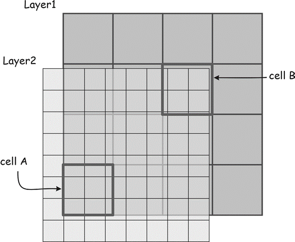
Figure 8: Incompatible cell sizes and boundaries confound multi-layer raster operations. This figure illustrates ambiguities in selecting input cell values from Layer2 in combination with Layer1. Multiple full and partial cells may contribute values for an operation applied to cell A. A portion of cell B is unde- fined in Layer2. These ambiguities are best resolved by resampling prior to layer combination. (source: Bolstad, 2016)

When layer extents differ, most GIS software will either restrict the operation to the area where input layers overlap. A null or a “missing data” number is usually assigned to cells where input data are lacking. This number acts as a flag, indicating there are no results. It is often a number, such as –9999, that will not occur from an operation, but any placeholder may be used as long as the software and users understand the place- holder indicates no valid data are present.

Incompatible raster cell sizes cause ambiguities when raster layers are combined (Figure 8). This problem is illustrated with an additional example here. Consider cell A in Figure 8 when Layer1 and Layer2 are combined in a raster operation. Several cells in Layer2 correspond to cell A in Layer1. If these two layers are added, there are likely to be several different input values for Layer2 corresponding to one input value for Layer1. The problem is compounded in cell B, because a portion of the cell is not defined for Layer2. It falls outside the layer boundary. Which Layer2 value should be used in a raster operation? Is it best to choose only the values in Layer2 from the cells with complete overlap, or to use the median number, the average cell number, or some weighted average? This ambiguity will arise whenever raster data sets are not aligned or have incompatible cell sizes. While the GIS software may have a default method for choosing the “best” input when cells are different sizes or do not align, these decisions are best controlled by the human analyst prior to the application of the raster operation.

As with vector operations, raster operations may be categorized as local, neighborhood, or global (Figure 9). Local operations use only the data in a single cell to calculate an output value. Neighborhood operations use data from a set of cells, and global operations use all data from a raster data layer. The concepts of local and neighborhood operations are more uniformly specified with raster data than with vector data. Cells within a layer have a uniform size, so a local operation has a uniform input area. In contrast, vector areas represented by polygons may have vastly different areas. Irregular polygonal boundaries cover differing areas and have differing footprints; for example, the local area defined by Alaska is different than the local area defined by Rhode Island. A local operation in a given raster is uniform in that it specifies a particular cell size and dimension.

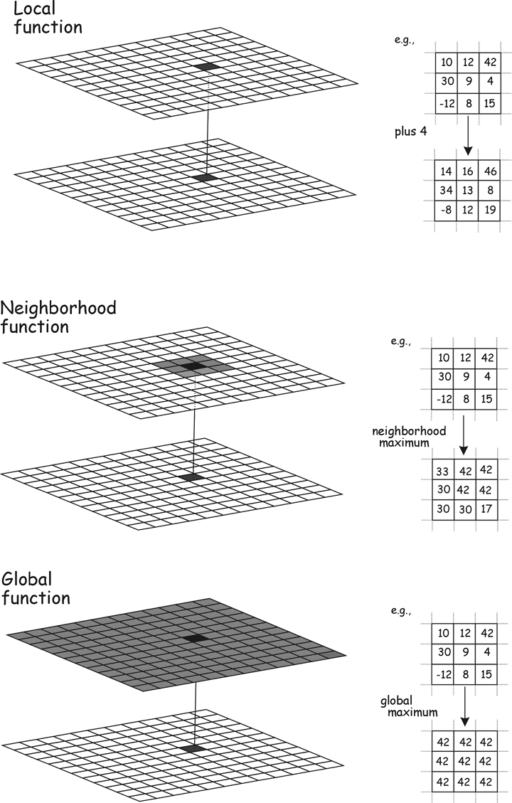
Figure 9: Raster operations may be local, neighborhood, or global. Target cells are shown in black, and source cells contributing to the target cell value in the output are shown in gray. Local operations show a cell-to-cell correspondence between input and output. Neighborhood operations include a group of nearby cells as input. Global operations use all cells in an input layer to determine values in an output layer. (source: Bolstad, 2016)

Neighborhood operations in raster data sets are also more uniformly defined than in vector data sets. A neighborhood may be defined by a fixed number of cells in a specific arrangement; for example, the neighborhood might be defined as a cell plus the eight surrounding cells. This neighborhood has a uniform area and dimension for most of the raster, with some minor adjustments needed near the edges of the raster data

layer. Vector neighborhoods may depend not only on the shape and size of the target fea- ture, but also on the shape and sizes of adja- cent vector features. Global operations in map algebra may produce uniform output, or they may pro- duce different values for each raster cell. Global operations that return a uniform value are in effect returning a single number that is placed in every cell of the output layer. For example, the global maximum function for a layer might be specified as:

$Out_num = globalmax(In_layer)$

This would assign a single value to *Out_num$. The value would be the largest number found when searching all the cells of In_layer. This “collapsing” of data from a two-dimensional raster may reduce the map algebra to scalar algebra. Many other functions return a single global value placed in every cell for a layer, for example, the global mean, maximum, or minimum.

Global operations are at times quite useful. Consider an analysis of regional temperature. We may wish to identify the areas where daily maximum temperatures were warmer this year than the highest regional temperature ever recorded. This analysis might help us to identify the extent of a warming trend. We would first apply a maximum function to all previous yearly weather records. This would provide a scalar value, a single number representing the regional maximum temperature. We would then compare a raster data set of maximum temperature for each day in the current year against the “highest ever” scalar. If the value for a day were higher than the regional maximum, we would output a flag to a cell location. If it were not, we would output a different value. The final output raster would provide a map of the cells exceeding the previous regional maximum. Here we use a global operation first to create our single scalar value (highest regional temperature). This scalar is then used in subsequent operations that output raster data layers.

12.4.0.1 Local Functions

There is a broad number of local functions (or operations) that can be conveniently placed in one of four classes: mathematical functions, Boolean or logical operations, reclassification, and multilayer overlay.

Mathematical Functions

We may generate a new data layer by applying mathematical functions on a cell-by-cell basis to input layers (Figure 10, Table 1). Most functions use one input layer and create one output layer, but any number of inputs and outputs may be sup- ported, depending on the function.

A broad array of mathematical functions may be used, limited only by the constraints of the raster data model. Raster data value and type are perhaps the most common constraints. Most raster models store one data value in a cell. Each raster data set has a data type and maximum size that applies to each cell; for example, a two-byte signed integer may be stored. Mathematical operations that create non-integer values, or values larger than 32,768 (the capacity of a two-byte integer), may not be stored accurately in a two- byte integer output layer.

Most systems will do some form of automatic type conversion, but there are often limits on the largest values that can be stored, even with automatic conversion. Most raster GIS packages support a basic suite of mathematical functions (Table 1). Although the set of functions and function names differ among software packages, nearly all packages support the basic arithmetic operations of addition through division, and most provide the trigonometric functions and their inverses (e.g., sin, asin). Truncation, power, and modulus functions are also commonly supported, and vendors often include additional functions they perceive to be of special interest.

Table 1: Common local mathematical functions.

Function	Description
Add, subtract, multiply, divide	cell-by-cell combination with the arithmetic operation
ABS	Absolute value of each cell
EXP, EXP10, LN, LN10	Applies base e and base 10 exponentiation and logarithms
SIN, COS, TAN, ASIN, ACOS, ATAN	Apply trigonometric functions on a cell-by-cell basis
INT, TRUNC	Truncate cell values, out- put integer portion
MODULUS	Assigns the decimal por- tion of each cell
ROUND	Rounds a cell value up or down to nearest integer value
SQRT, ROOT	Calculates the square root or specifies other root of each cell value

Examples of addition and multiplication functions are shown in Figure 10. We will not show additional examples because most differ only in the function that is applied. These mathematical functions are often applied in raster analysis, for example, when multiplying each cell by 3.28 to convert height values from units in meters to units measured in feet.

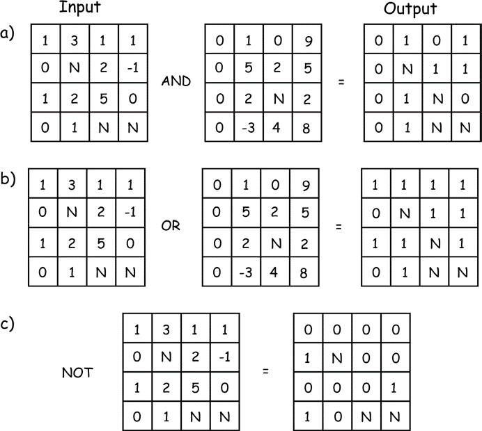
Figure 10: Examples of logical operations applied to raster data. Operations place true (non-zero) or false values (0) depending on the input values. AND requires both correspond- ing input cells be true for a true output, OR assigns true if either input is true, and NOT sim- ply reverses the true and false values. Null or unassigned cells are denoted with an N. (source: Bolstad, 2016)

Note that although many systems will let you perform these operations on any type of raster data, they often only make sense for interval/ratio data, and may return erroneous results when applied to nominal or ordinal data. Numbers may be assigned to indicate population density by high, medium, and low, and while the sin function may be applied to these data, the results will usually have little meaning.

Logical Operations

There are many local functions that apply logical (also known as Boolean) operations to raster data. A logical operation typically involves the comparison of a cell to a scalar value or set of values and outputs a “true” or a “false” value. True is often represented by an output value of 1, and false by an output value of 0.

There are three basic logical operations, AND, OR, and NOT (Figure 10). The AND and OR operations require two input layers. These layers serve as a basis for comparison and assignment. AND requires both input values be true for the assignment of a true output. Typically, any nonzero value is considered to be true, and zeros false. Note in Figure 10-4a that output values are typically restricted to 1 and 0, even though there may be a range of input values. Also note that there may be cells where no data are recorded. How these are assigned depends on the specific GIS system. Most systems assign null output when any input is null; others assign false values when any input is null.

Figure 10b shows an example of the OR operation. This cell-by-cell comparison assigns true to the output if either of the cor- responding input cells is true. Note that the cells in either layer or both layers may be true for a true assignment, and that in this example, null values (N) are assigned when either of the inputs is null. Some implementations assign a true value to the output cell if any of the inputs is non-null and nonzero; the reader should consult the manual for the specific software tool they use. Figure 10-4c shows an example of the NOT operation. This operation switches true for false, and false for true. Note that null input assigns null output. Finally, note that many systems provide an XOR operation, known as an eXclusive OR (not illustrated in our examples). This is similar to an OR operation, except that true values are assigned to the output when only one or the other of the inputs is true, but not when both inputs are true. This is a more restrictive case than the general OR, and

may be used in instances when we wish to distinguish among origins for a true assignment. Logical operations may be provided that perform ordinal or equality comparisons, or that test if cell values are null (Figure 11). Ordinal comparisons include less than, greater than, less than or equal to, greater than or equal to, equal, and not equal. Examples of these logical comparisons are shown in Figure 10-5a and b, respectively. These operations are applied cell-by-cell, and the corresponding true or false output assigned. As shown in Figure 10-5a, the upper left cell of the first input layer is not less than the upper left cell of the second input layer, so a 0 (false) is assigned to the upper left cell in the output layer. The upper right cell in the first layer is less than the cor- responding cell in the second input layer, resulting in the assignment of 1 (true) in the output layer.

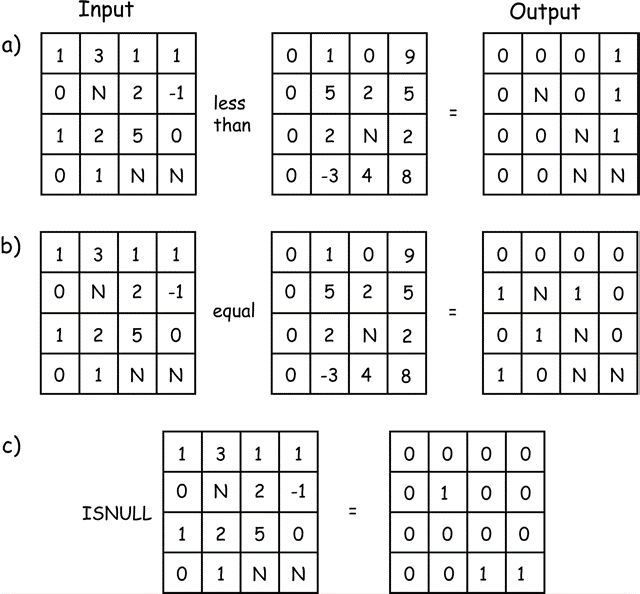
Figure 11: Examples of logical comparison operators for raster data sets. Output values record the ordinal comparisons for inputs, with a 1 signifying true and a 0 false. The ISNULL operation assigns true values to the output whenever there are missing input data. (source: Bolstad, 2016)

We often need to test for missing or unassigned values in a raster data layer. The operation has no standard name, and may be variously called via ISMISSING, ISNULL, or some other descriptive name. The operation tests each cell for a null value, shown as N in Figure 10-5c. A 0 is assigned to the cor- responding output cell if a non-null value is found, otherwise a 1 is assigned. These tests for missing values are helpful when identifying and replacing missing data, or when determining the adequacy of a data set and identifying areas in need of additional sampling.

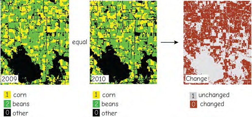
Figure 12: An example of a logical operation applied to categorical data, here landuse classes of corn (value = 1), soybeans (2), and other crops (0) over two time periods. The equal operation returns 0 where land use has changed, and 1 where it has remained constant over these two periods. (source: Bolstad, 2016)

Figure 12 shows an example of a logical comparison among two data layers. The left and central panels show landcover for an agricultural area, with three categories: corn (1), soybeans (2), and all others (0). We may be interested in identifying acres that were rotated between these two crops, or from these two crops to other crops over the 2009- 2010 time period. The logical equal comparison between these layers reveals areas that have changed. If the cell values are not equal across the years, the logical equal comparison will return a value of 0, while areas that remain the same will maintain the value of 1. Further logical comparisons, using class val- ues, could identify how much each of the component crop types had changed.

Note that logical operators may be applied to interval/ratio, ordinal, and cate- gorical data, although ordinal comparisons should be carefully applied to categorical data. For example, in our crop types example in Figure 10-6, soybeans are assigned a value of 2, and are “larger” than corn, but this distinction does not imply that soybeans are somehow two times larger, more valu- able or anything other than just different from corn.

Reclassification

Raster reclassification assigns output values that depend on the specific set of input values. Assignment is most often defined by a table, ranges of values, or a conditional test. Raster reclassification by a table is based on matching input cell values to a reclassification table (Figure 13a). The reclassification table specifies the mapping between input values and output values.

Each input cell value is compared to entries for an “in” column in the table. When a match is found, the corresponding “out” value is assigned to the output raster layer. Unmatched input values can be handled in one of several ways. The most logically con- sistent manner is to assign a null value, as shown in Figure 13a for the input value of -1. Some software simply assigns the input cell value when there is no match. As with all spatial processing tools, the specifics of the implementation must be documented and understood.

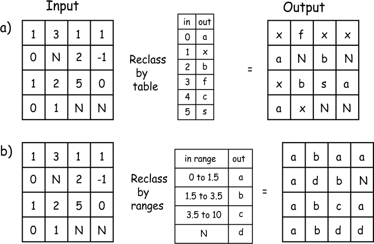
Figure 13: Raster reclassification by table matching (a) and by table range (b). In both cases, input cell values are compared to the “in” column of the table. A match is found and the corre- sponding “out” values assigned. (source: Bolstad, 2016)

Figure 13b illustrates a reclassification by a range of values. This process is similar to a reclassification by a table, except that a range of values appears for each entry in the reclassification table. Each range cor- responds to an output value. This allows a more compact representation of the reclassification. A reclassification over a range is also a simple way to apply the automated reclassification rules discussed at length — the equal interval, equal area, natural breaks, or other automated class-creation methods. These automated assignment methods are often used for raster data sets because of the large number of values they contain.

Data can also be reclassified to select the input source based on a condition. These “conditional” functions have varying syntax, but typically require a condition that results in a true or false outcome. The value or source layer assigned for a true outcome is specified, as is the value or source layer assigned for a false outcome. An example of one conditional function may be:

$Output = CON (test, out if true, out if false)$

where CON is the conditional function, test is the condition to be tested, out if true defines the value assigned if the condition tests true, and out if false defines the value assigned if the condition tests false (Figure 14). Note that the value that is output may be a scalar value, for example, the number 2, or the value output may come from the corresponding location in a specified raster layer. The condition is applied on a cell-by- cell basis, and the output value assigned based on the results of the conditional test.

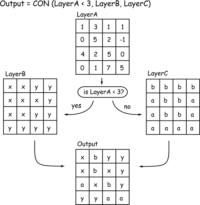
Figure 14: Reclassification by condition assigns an output based on a conditional test. In this example, each cell in LayerA is compared to the number 3. For Layer A cells with values less than 3, the condition evaluates to true, and the output cell value is assigned from LayerB. If the LayerA cell value is equal to or greater than 3, then the output cell value is assigned from LayerC. (source: Bolstad, 2016)

Neighborhood, Zonal, Distance, and Global Functions

Neighborhood functions (or operations) in raster analyses deserve an extended dis- cussion because they offer substantial ana- lytical power and flexibility. Neighborhood operations are applied in many analyses across a broad range of topics, including the calculation of slope, aspect, and spatial cor- relation.

Neighborhood operations most often depend on the concept of a moving window. A “window” is a configuration of raster cells used to specify the input values for an operation (Figure 15). The window is positioned on a given location over the input raster, and an operation applied that involves the cells contained in the window. The result of the operation is usually associated with

the cell at the center of the window position. The result of the operation is saved to an out- put layer at the center cell location. The win- dow is then “moved” to be centered over the adjacent cell and the computation repeated (Figure 15). The window is swept across a raster data layer, usually from left to right in successive rows from top to bottom. At each window location the moving window function is calculated and the result output to the new data layer.

Figure 15: The concept of a moving window in raster neighborhood operations. Here a 3 by 3 window is swept from left to right and from top to bottom across a raster layer. The window at each location defines the input cells used in a raster operation. (source: Bolstad, 2016)

Moving windows are defined in part by their dimensions. For example, a 3 by 3 moving window has an edge length of three cells in the x and y directions, for a total area of nine cells. Moving windows may be any size and shape, but they are typically odd-numbered in both the x and y directions to provide a natural center cell, and they are typically square. A 3 by 3 cell window is the most common size, although windows may also be rectangular. Windows may also have irregular shapes; for example, L-shaped, circular, or wedge-shaped moving windows are sometimes specified.

There are many neighborhood functions that use a moving window. These include simple functions such as mean, maximum, minimum, or range (Figure 16). Neighborhood functions may be complicated, for example, the statistical standard deviation, and they may be non-arithmetic, as the functions that returns a count of the number of unique values, or the mode, or a Boolean occurrence. Any function that combines information from a consistently shaped group of raster cells may be implemented with a moving window. Moving window functions may be arithmetic, adding, subtracting, averaging, or otherwise mathematically combining the values around a central cell, or they may be com- parative or otherwise extract values from a set of cells. Common statistical operations include calculating the largest value, the mode (peak of a histogram), median (middle value), the range (largest minus smallest), or diversity (number of different values). These neighborhood operations are useful for many kinds of processing.

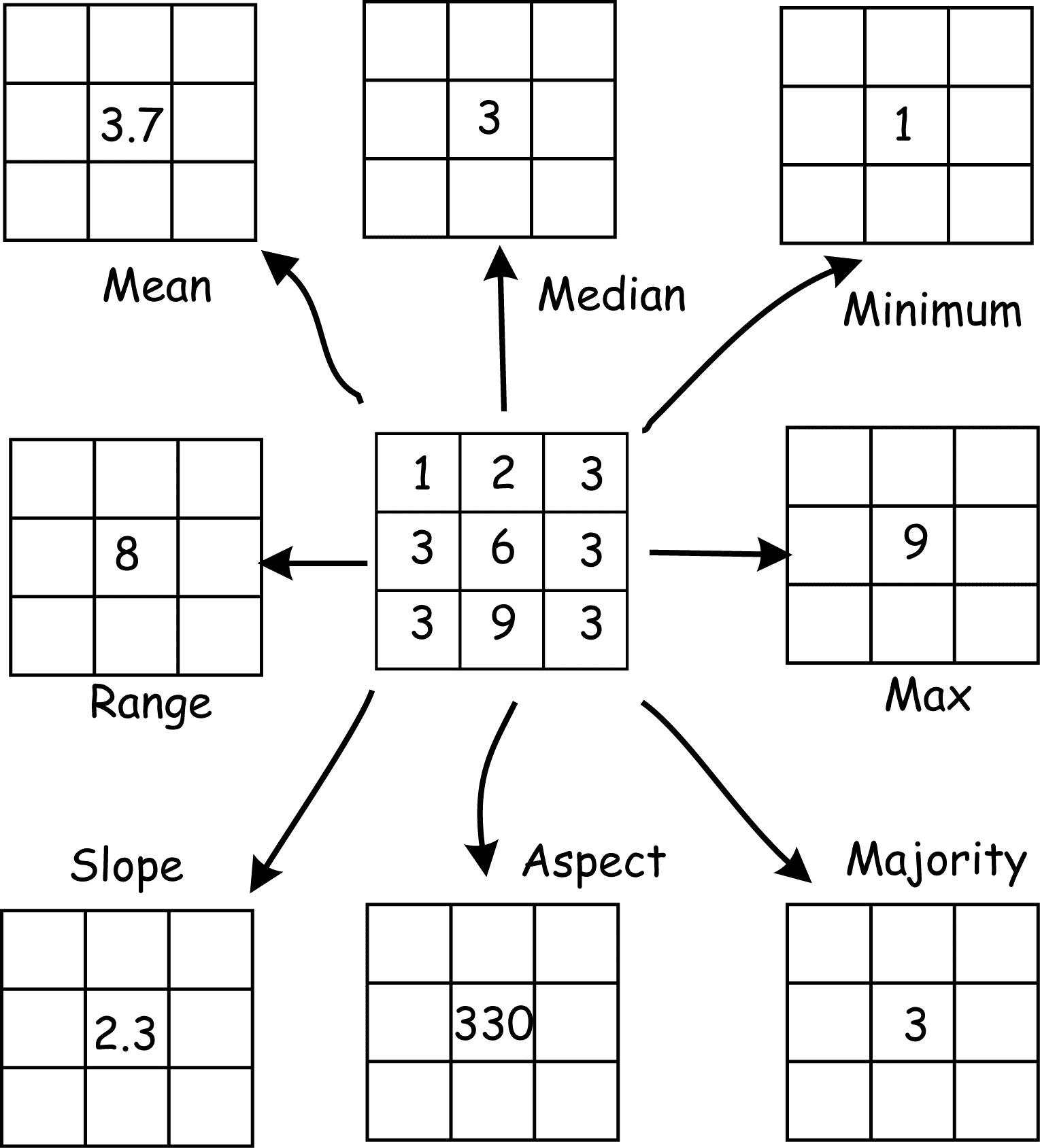
Figure 16: A given raster neigh- borhood may define the input for several raster neighborhood opera- tions. Here a 3 by 3 neighborhood is specified. These nine cells may be used as input for mean, median, minimum, or a number of other functions. (source: Bolstad, 2016)

Consider the majority operation, also known as a majority filter. You might wonder why one would want to calculate a majority filter for a data layer. Data smoothing is a common application. We described in Chapter 6 how multi-band satellite data are often converted from raw image data to landcover classification maps.These classifiers often assign values on a pixel basis, and often result in many single pixels of one landcover type embedded within another landcover type. These single pixels are often smaller than the minimum mapping unit, the smallest uniform area that we care to map. A majority filter is often used to remove this classification “noise.”

A majority filter is illustrated in Figure 17. It illustrates NASS crop data for an area in central Indiana, based on classified satellite images. There are over 40 common landcover types in the area, but these have been reclassified into the dominant types of developed (road), corn, beans, and other crops. Each pixel is 30 m across, and the image on the left is NASS data as delivered. Note that corn and beans dominate, but there are many “stray” pixels of a dissonant vegetation type embedded or on the edge of a dominant type in an area; for example, bean pixels in a corn field, or corn pixels in a bean field. These stray pixels usually do not rep- resent reality, in that although there may be the isolated plant or two from previously deposited seed in these annual crop rotations, the patches almost never approach 30 meters in size. The embedded cells are most often misclassifications due to canopy thinning or perhaps weeds below the crop, and are often below the minimum mapping unit.

The illustrated majority filter counts the values of the four cells sharing an edge with any given cell. If a majority, meaning three or more cells, are of a type, then the cell is output as this majority type (top, Figure 17). If a majority is not reached, as when only one or two cells add up to the most frequent type in the four bordering cells, then the center cell value is unchanged in the out- put (Figure 10-17). The removal of most of the single pixel “noise” by the majority filter can be observed in the classified image on the right side of Figure 17.

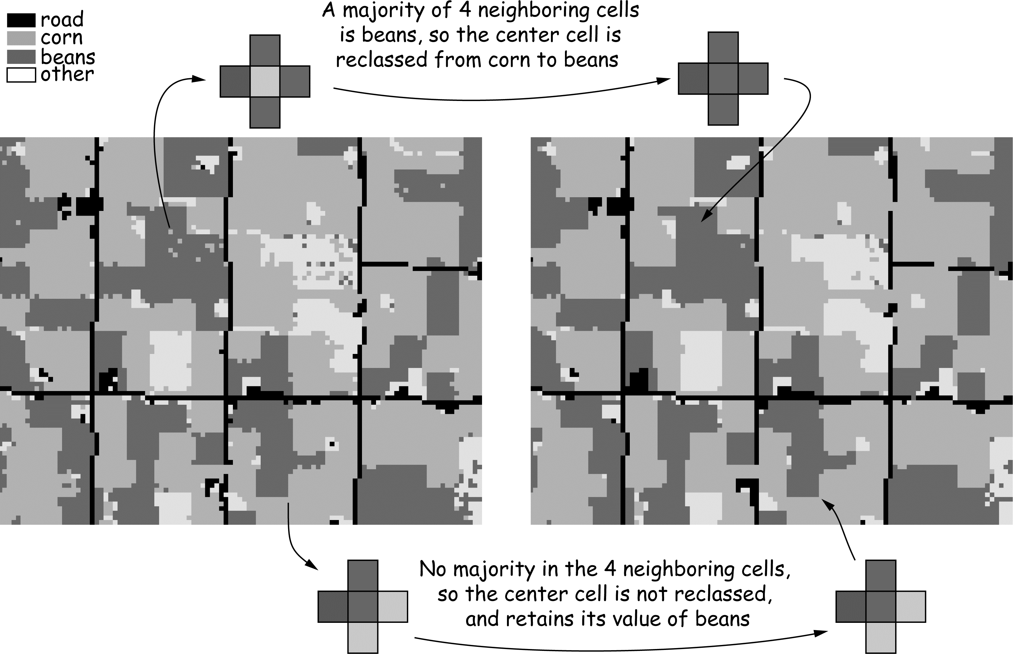
Figure 17: An example of a majority filter applied to a raster data layer from a classified satellite image. Many isolated cells are converted to the category of the dominant surrounding class. (source: Bolstad, 2016)

There may be many variants for a given operation. The majority filter just discussed may assign an output value if only two of the four adjacent cell values are most frequent, or use the 8 or 24 nearest cells to calculate a majority. The dependence of output on algo- rithm specifics should always be recognized when applying any raster operation.

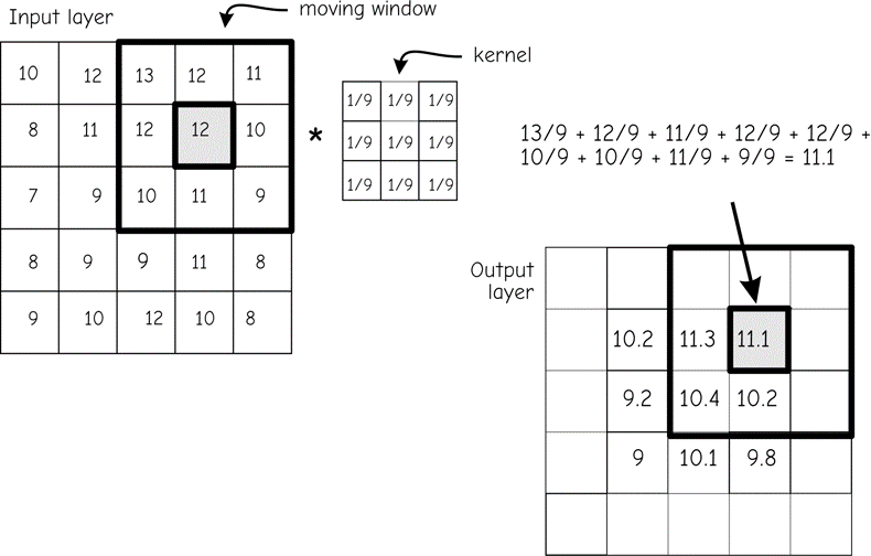
Figure 18: An example of a mean function applied via a moving window. Input layer cell values from a 3 by 3 moving window (upper left) are multiplied by a kernel to specify corresponding output cell val- ues. This process is repeated for each cell in the input layer. (source: Bolstad, 2016)

Figure 18 shows an example of a mean calculation using a moving window. The function scans all nine values in the window. It sums them and divides the sum by the number of cells in the window, thus calculating the mean cell value for the input window. The multiplication may be represented by a 3 by 3 grid containing the value one-ninth (1/9). The mean value is then stored in an output data layer in the location corresponding to the center cell of the mov- ing window. The window is then shifted to the right and the process repeated. When the end of a row is reached the window is returned to the leftmost columns, shifted down one row, and the process repeated until all rows have been included.

The moving window for many simple mathematical functions may be defined by a kernel. A kernel for a moving window function is the set of cell constants for a given window size and shape. These constants are used in a function at every moving window location. The kernel in Figure 18 specifies a mean. As the figure shows, each cell value for the Input layer at a given window position is multiplied by the corresponding kernel constant. The result is placed in the Output layer.

Note that when the edge of the moving window is placed on the margin of the original raster grid, we are left with at least one border row or column for which output values are undefined. This is illustrated in Figure 18. The moving window is shown in the upper right corner of the input raster. The window is as near the top and to the right side of the raster as can be without placing input cell locations in the undefined region, outside the boundaries of the raster layer.

The center cell for the window is one cell to the left and one cell down from the corner of the input raster. Output values are not defined for the cells along the top, bottom, and side margins of the output raster when using a 3 by 3 window, because a portion of the moving window would lie outside the raster data set. Each operation applied to successive output layers may erode the mar- gin further. There are several common methods of addressing this margin erosion. One is to define a study area larger than the area of interest. Data may be lost at the margins, but these data are not important if they are out- side the area of interest. A second common approach defines a different kernel for mar- gin windows (Figure 19). Margin kernels are similar to the main kernels, but modified as needed by the change in shape and size. Figure 19 illustrates a 3 by 3 kernel for the bulk of the raster. Corner values may be determined using a 2 by 2 kernel, and edges can be determined with 2 by 3 kernels. Out- puts from these kernels are placed in the appropriate edge cells.

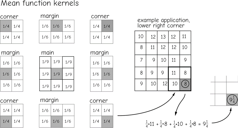
Figure 19: Kernels may be modified to fill values for a moving window function at the margin of a ras- ter data set. Here the margin and corner kernels are defined differently than the “main” kernel. Output val- ues are placed in the shaded cell for each kernel. The margin and corner kernels are similar to the main kernel, but are adjusted in shape and value to ignore areas “outside” the raster.(source: Bolstad, 2016)

Different moving windows and kernels may be specified to implement many different neighborhood functions. For example, kernels may be used to detect edges within a raster layer. We might be interested in the difference in a variable across a landscape. For example, a railway accident may have caused a chemical spill and seepage through adjacent soils. We may wish to identify the boundary of the spill from a set of soil samples. Suppose there is a soil property, such as a chemical signature, that has a high concentration where the spill occurred, but a low concentration in other areas. We may apply kernels to identify where abrupt changes in the levels of this chemical create edges.

Edge detection is based on comparing differences across a kernel. The values on one side of the kernel are subtracted from the values on the other side. Large differences result in large output values, while small differences result in small output values. Edges are defined as those cells with output values larger than some threshold.

Figure 20 illustrates the application of an edge detection operation. The kernel on the left side of Figure 20 amplifies differences in the x direction. The values in the left of three adjacent columns are subtracted from the value in the corresponding right-hand row of cells. This process is repeated for each cell in the kernel, and the values summed across all nine cells. Large differences result in large values, either positive or negative, saved in the center cell. Small differences between the left and right columns lead to a small number in the center cell.

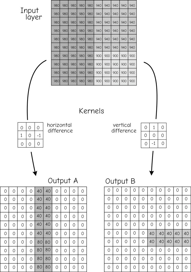
Figure 20: There is a large number of kernels used with moving windows. The kernel on the left amplifies differences in the x direction, while the kernel on the right amplifies differences in the y direc- tion. These and other kernels may be used to detect specific features in a data layer.(source: Bolstad, 2016)

Thus, if there are large differences between values when moving in the x direction, this difference is highlighted. Spatial structure such as an abrupt change in elevation may be detected by this kernel. The kernel in the middle-right of Figure 20 may be used to detect differences in the y direction. Neighborhood functions may also smooth the data. An averaging kernel, described above in Figure 18 and Figure 19, will reduce the difference between a cell and surrounding cells. This is because windows average across a group of cells, so there is much similarity in the output values calculated from adjacent window placements.

Raster data may contain “noise.” Noise are values that are large or small relative to their spatial context. Noise may come from several sources, including measurement errors, mistakes in recording the original data, miscalculations, or data loss. There is often a need to correct these errors. If it is impossible or expensive to revisit the study area and collect new data, the noisy data may be smoothed using a kernel and moving window.

There are functions known as high-pass filters with kernels that accentuate differences between adjacent cells. These high- pass filter kernels may be useful in identifying the spikes or pits that are characteristic of noisy data. Cells identified as spikes or pits may then be evaluated and edited as appropriate, removing the erroneous values. High-pass kernels generally contain both negative and positive values in a pattern that accentuates local differences.

Figure 21 demonstrates the use of a high-pass kernel on a data set containing noise. The elevation data set shown in the top portion of the figure contains a number of anomalous cells. These cells have extremely high values (spikes, shown in black) or low values (pits, shown in white) relative to nearby cells. If uncorrected, pits and spikes will affect slope, aspect, and other terrain-based calculations. These locally extreme values should be identified and modified. The high-pass kernel shown contains a value of 9 in the center and -1 in all other cells. Each value is divided by 9 to reduce the range of the output variable. The kernel returns a value near the local average in smoothly changing areas. The positive and negative values balance, returning small numbers in flat areas.

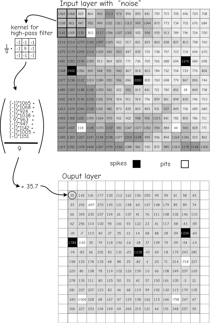
Figure 21: An example of a moving window function. Raster data often contain anomalous “noise” (dark and light cells). A high-pass filter and kernel, shown at top left, highlights “noisy” cells. Local differ- ences are amplified so that anomalous cells are easily identified. (source: Bolstad, 2016)

The high-pass kernel generates a large positive value when centered on a spike. The large differences between the center cell and adjacent cells are accentuated. Conversely, a large negative value is generated when a pit is encountered. An example shows the application of the high-pass filter for a cell near the upper left corner of the input data layer (Figure 21). Each cell value is multiplied by the corresponding kernel coefficient.

These numbers are summed, and divided by 9, and the result placed in the corresponding output location. Calculation results are shown as real numbers, but cell values are shown here recorded as integers. Output val- ues may be real numbers or integers, depending on the programming algorithm and perhaps the specifications set by the user.

The mean filter is representative of many moving window functions in that it increases the spatial covariance in the out- put data set. High spatial covariance means values are autocorrelated (discussed in greater depth when in the spatial prediction section of Chapter 13). A large positive spatial covariance means cells near each other are likely to have similar values. Where you find one cell with a large number, you are likely to find more cells with large numbers. If spatial data have high spatial covariance, then small numbers are also likely to be found near each other. Low spatial covariance means nearby values are unrelated – knowing the value at one cell does not provide much information about the values at nearby cells. High spatial covariance in the “real world” may be a good thing. If we are prospecting for minerals then a sample with a high value indicates we are probably near a larger area of ore-bearing deposits. However, if the spatial autocorrelation is increased by the moving window function we may get an overly optimistic impression of our likelihood of striking it rich.

The spatial covariance increases with many moving window functions because these functions share cells in adjacent calculations. Note the average function in Figure 22. The left of Figure 22 shows sequential positions of a 3 by 3 window. In the first window location the mean is calculated and placed in the output layer. The window center is then shifted one cell to the right, and the mean for this location calculated and placed in the next output cell to the right. Note that there are six cells in common for these two means. Adjacent cells in the output data layer share six of nine cells in the mean calculation. When a particularly low or high cell occurs, it affects the mean of many cells in the output data layer. This causes the outputs to be quite similar, and increases the spatial covariance.

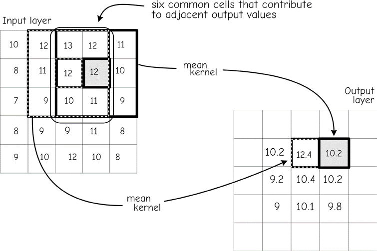
Figure 22: A moving window may increase spatial covariance. Adjacent output cells share many input cell values. In the mean function shown here, this results in similar output cell values. (source: Bolstad, 2016)