4 Raster data

The basis of raster data is the overlap of the studied entity or area with a regular network (grid). The entity is then described by discrete values that are related to the fields of this network. The positional location of an entity is determined by the coordinates of the fields that represent it (Figure 1).

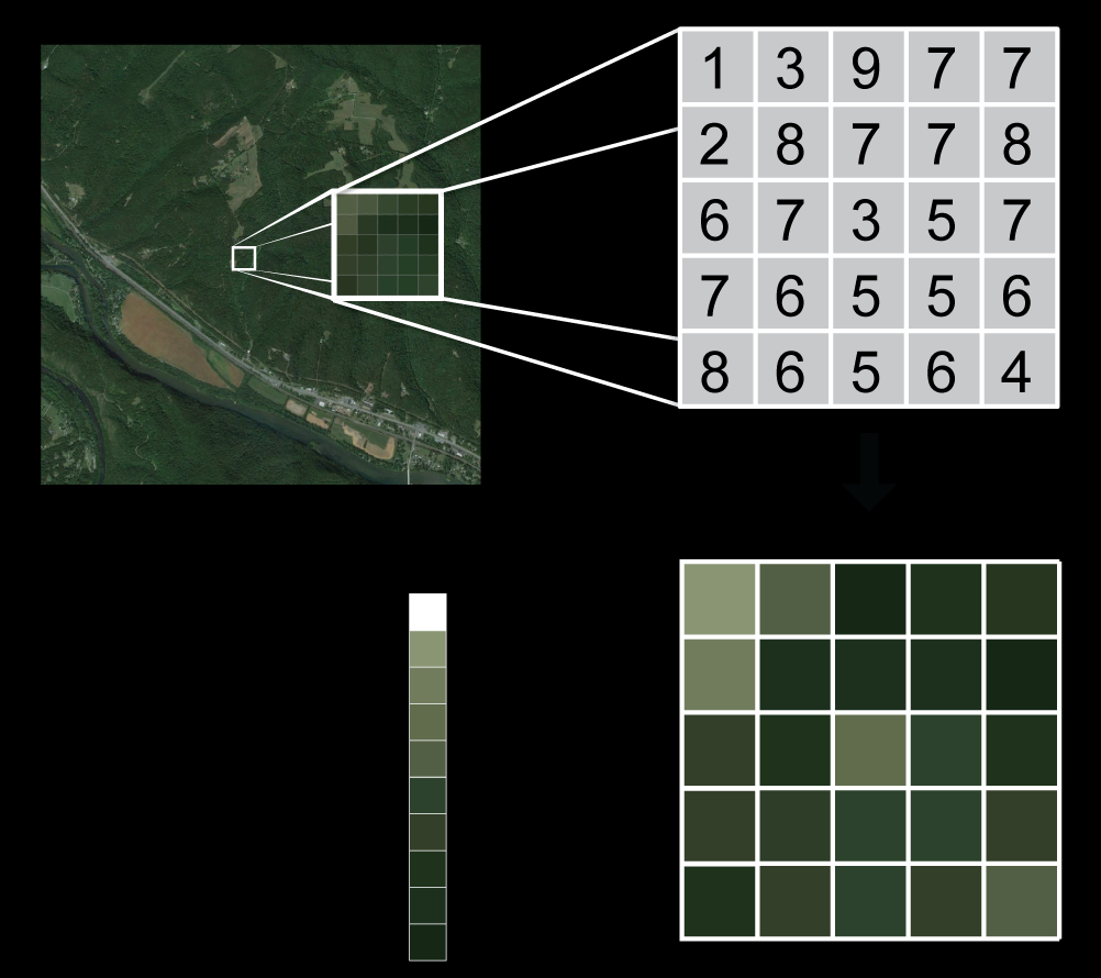
Figure 1: Raster data concept (source: https://datacarpentry.org/organization-geospatial/01-intro-raster-data/)

Raster data are especially suitable for the representation of continuous phenomena, such as:

• air and water temperature,
• altitude,
• geological data,
• precipitation map,
• surface runoff density,
• aerial and satellite imagery and more.

The basic shape of a cell is derived from basic geometric shapes that meet the rules:

• infinite divisibility of a cell into cells of the same shape and
• the ability to fill a defined area without rest and without overlap by arranging cells side by side.

From the stated requirements for the basic shape of the cell, this is met by a square, rectangular and triangular cell. In GIS software applications, the raster is usually formed by a matrix of square cells. Raster size (range), its height and width are determined by the number of columns and rows in the matrix and the spatial resolution of the cell. The rows and columns are usually perpendicular to each other and are usually oriented parallel to the axes of the Cartesian coordinate system.

Each raster must be connected to the coordinate system (georeference). This is done by defining coordinates for the reference point (center or corner of at least one cell) of the raster. If the raster is not connected to the coordinate system via a reference point, the raster has only so-called image coordinates. I.e. the position of each cell can only be described by an index number describing the position of the cell within the raster matrix, relative to the reference point. Image coordinates are impractical for most GIS applications. Therefore, in the absence of real coordinates, a geometric transformation of the image coordinates to real coordinates is performed.

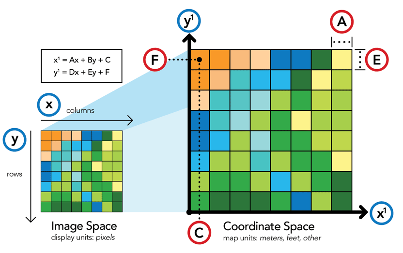
Figure 2: Raster georeferrencing (source: https://www.esri.com/about/newsroom/arcuser/understanding-raster-georeferencing/)

Depending on the format that is chosen to store the raster data, one raster file may contain multiple subimages with identical basic raster matrix parameters. Each of the sub-images then differs in the values contained in its cells. The name band is used for these sub-rasters (Figure 3). When displaying these rasters, a combination of three bands is always displayed, where each band is displayed using one color channel RGB. This approach is very often used for digital imagery taken by satellites or digital aerial imagery.

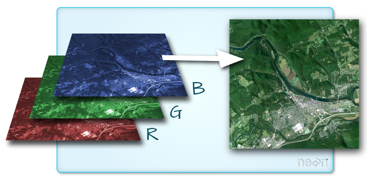
Figure 3: Multi-band raster (source: https://www.neonscience.org/dc-multiband-rasters-r)

An overview of raster formats used in Geoinformatics can be found in GDAL00.

4.1 Types of space division

There are two basic ways to divide a space (Figure 4):

• regular division of space - the shape of the cells is precisely defined and always the same - square, rectangle, hexagon, triangle. These rasters are further divided into
  • rasters with the same resolution level - individual cells are the same size
  • rasters with unequal resolution level or hierarchical - cell size changes in a defined way.
• irregular division of space, in which cells of different shape and size are formed.

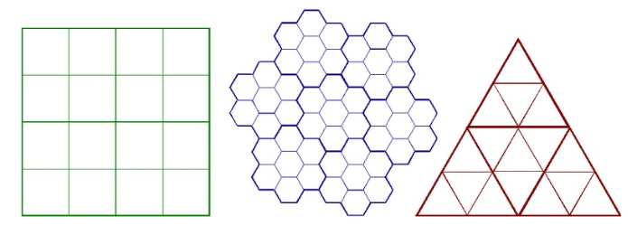
Figure 4: Different divisions of space in rasters

Practical applications consist mainly in the use of regular tessellations (mosaics), mainly with the same level of resolution. Hierarchical structures are sometimes understood more as data compression methods. Historically, square rasters are the most used, mainly for the following reasons:

• are compatible with data structures used in computer technology (matrices),
• are compatible with many hardware devices for data recording and output (scanners, printers, plotters),
• are compatible with Cartesian coordinate systems.

Only square-shaped cells can be divided into smaller squares with the same shape and orientation. The basic spatial cells of a raster are called raster cells or pixels - picture element. The three-dimensional variant of a pixel is called voxel. Sometimes the terms are confused, e.g. the term “raster” is used to mean “raster cell”, but in the true sense of the word, raster means a system at right angles of intersecting lines that delimit individual cells. If we take into account the system of intersections of these lines, it is a point raster - lattice. In a point grid, thematic data refer to the exact position in space, in a cell grid, to the part of the area represented by a cell element.

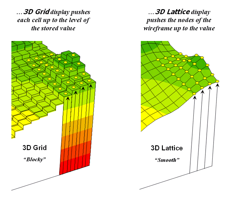
Figue 5: Area and point raster in 3D (source: https://blogs.ubc.ca/advancedgis/schedule/slides/spatial-analysis-2/lattices-vs-grids/)

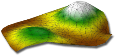
The main advantage of a hexagonal grid is that the centers of all adjacent cells are equidistant from the center of the cell. This symmetry makes the model advantageous for some analytical functions, such as radial scanning, which is not possible with a square or triangular network. However, hexagonal cells are rarely used in practice. The basic characteristic of all triangular tessellations is that the triangles do not have the same orientation, which is advantageous for representations of terrain and other surfaces. Triangles of variable size and shape are most often used for these purposes, so-called triangular irregular network (TIN).

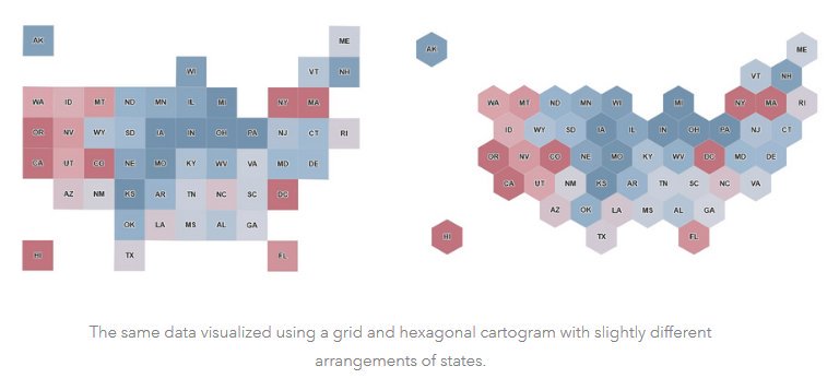
Figure 6: Square and hexagonal raster (source: https://twitter.com/GIS_Bandit/)

Raster cell topology is implicitly defined in raster geometry. Each pixel has two types of neighbors:

• full - perfect (full) neighbors - adjacent pixels in the same rows or columns - these cells create so-called four-member (von Neumann) neighborhood;
• diagonal neighbors - pixels that touch a given person in its corners;
• Both groups of neighbors create so-called eight-member (Moore) neighborhood.

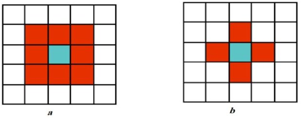
Figure 8: Moore (a) and von Neumann (b) cell surroundings (source: Gazmeth et al., 2013)

4.1.1 Factors affecting the quality of the real-world raster display

The quality of the real-world display using a raster data model is affected by several factors:

• the method of assigning the values of the displayed attribute to individual cells,
• spatial resolution - size of the basic cell of the raster,
• color resolution - the number of values that a pixel can take (record attribute values), legally called in the case of a digital image "radiometric resolution in ESRI help, this number is then called the Bit Depth.
  
  

How to assign the values of the displayed attribute to individual cells

Attribute values in individual cells can be determined in different ways:

• as a point value measured anywhere in the cell area,
• as an arithmetic mean of several point measurements,
• as a weighted arithmetic mean, where the weight is the area of individual values,
• as the maximum or minimum value of the attribute,
• as the value of the attribute with the highest weight.

The choice of a specific method of assigning the values of a given attribute to individual cells can significantly affect the resulting representation of the area of interest in growth, both in terms of boundaries with different values of the observed attribute, and in terms of representation of small areas.

Figure 9 shows possible ways to assign values to a cell if multiple land use categories fall into that cell.

Figure 9: The problem of assigning a value to a cell with multiple categories

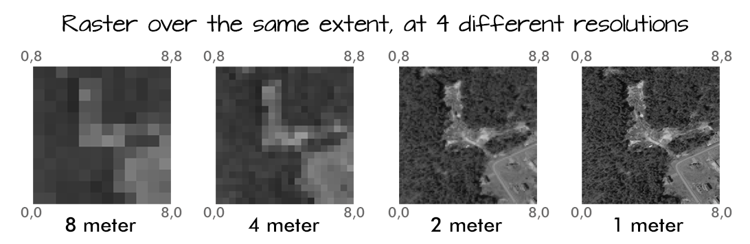
The size of the raster base cell

In general, the smaller the basic cell of the raster, the better (more accurately) the course of the boundaries of individual geoelements can be captured in this raster (Figure 10). However, the same is true: halving the side length of the raster base cell quadruples the memory space required to store the raster.

“Color depth” (resolution) of the raster

When working with rasters, we use different resolutions in individual cells to record the values of the monitored attribute. According to the resolution used, we distinguish the following types of rasters:

• binary - only the presence or absence of attribute (most often values 0 and 1) - to record the value of one cell we always need one bit - e.g. scanned cadastral maps.
• 8-bit - we distinguish 256 different integer values of the monitored attribute in the cell - to record the value of one raster cell we need 1 Byte - eg scanned color masters, panchromatic aerial and satellite images.
• twenty-four-bit - there are about 1.6 million different integer values of the monitored attribute in the cell - to record one cell we need 3 bytes - eg multispectral satellite images.
• continuous - in the cell we distinguish an almost unlimited number of real values of the monitored attribute - to record one cell we usually need 4, resp. 6 Byte.

In practice, the first three types of rasters are most often used. Binary rasters are used when working with scanned cadastral maps, the source of 8-bit rasters are mainly scanned color masters and panchromatic aerial and satellite images, or they are produced by raster systems in common raster analyzes. Twenty-four-bit rasters are most often created as a product of multispectral satellite image processing.

4.2 Qualitative and quantitative rasters and raster formats

Quantitative raster shows the quantity of the observed phenomenon. It therefore describes the magnitude of the phenomenon recorded in a given cell. Cells can take real number values. The values used in the quantitative raster are usually from the ratio or interval domain. This type of raster is characterized by a large variability of values. Examples of quantitative rasters are shown in Figures 11. Most GIS software applications have their own native format for storing this type of raster.

Formats for storing quantitative data: TIFF, GeoTIFF, BIL, BIP, BSQ, ArcInfo Grid (Binary, ASCII), RST (IDRISI), IMG (Erdas Imagine), GRD (Intergraph Raster Format).

Qualitative raster expresses the quality (type, kind, class, category) of the phenomenon. Cells carry an integer value. Usually, this value can only be positive, but it is not an unconditional rule. The cell values used in these rasters are from the enumerated (nominal) domain. The variability of values in this raster is relatively small, rarely exceeding the number of values of the first 100 values.

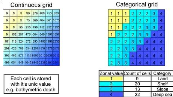
Figure 11: Quantitative and categorial raster (source: https://is.muni.cz/el/1431/jaro2017/Z0262/um/geoinformatika_03_fin.pdf)

Quantitative rasters can be divided into rasters that represent thematic data, actual enumerated values such as land use type, and image record rasters that are used to store satellite data, aerial photography data, scanned intermediates, or maps.

In the field of Geoinformatics, image data are often used as a topographic basis or as a source for further subsequent processing, for example in the form of thematic rasters or quantitative rasters. An example of an Image raster can be: an aerial image, a satellite recording, or a digital raster copy of an analog map. This data is either displayed as three-channel (RGB), with the files themselves containing tens to hundreds of bands.

Formats for storing image data: TIFF, JPEG, PNG, BMP, MrSID, ECW, BIL, BIP, BSQ + proprietary formats of manufacturers listed for quantitative raster data.

4.3 Triangulation

A large number of triangular networks can be created from a certain set of entry points. This procedure is called triangulation. The so-called Delaunay triangulation is of great importance (see Figure 12). Triangulation is Delaunay triangulation just when no other point falls into the circle circumscribed to each of the triangles. The vertex of each triangle of the network is bounded by a convex triangle.

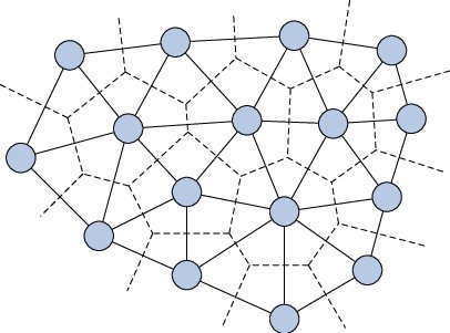
Figure 12: Delaunay triangulation and Voronoi diagram (source: DalleMole et al., 2010)

The duality of this triangulation is called the Voronoi diagram or Thiessen polygons or Dirichlet tesselation. The vertices of the Voronoi polygons are also the centers of the circles circumscribed by the Delaunay triangles. The perpendiculars leading to the centers of the sides of the Delaunay triangulation form the edges of the Voronoi polygons. Since Delaunay triangulation and Voronoi polygons form a duality, Delaunay triangulation can be created from Voronoi polygons and vice versa. The requirement of “absence of a point in a circle circumscribed by the triangles of a network” is called the empty circle criterion or the Delaunay criterion.

If we define a raster cell as an indivisible basic unit of space, the raster model no longer needs a continuous coordinate system. Discrete raster space will suffice. As a result, we do not need a pair of coordinates to describe the position in the raster. A pair of indices \(i, j\) is sufficient to define the position of the cell with respect to the beginning of the raster. The use of index j as the index of rows of raster cells and index i as the index of raster cell shells is introduced. Compared to a vector model, this type of position description is very simple. Instead of real coordinates, we use integer variables as indices. This fact is very important in terms of the required memory space.

Indices can be calculated from coordinates according to the following rules:

\(X_{1}\rightarrow i=0\)

\(Y_{1}\rightarrow j=0\)

\(X=X_{1}+p\cdot \delta X \rightarrow i=p\)

\(Y=Y_{1}+q\cdot \delta Y \rightarrow j=q\),

where $ delta X $, $ delta Y $ are the step distance sizes (raster base cell dimensions) that determine the raster resolution. Reducing them increases the resolution. Coordinates from indices can be calculated using the above rules.

The processing time for most raster operations depends on their resolution, more or less increasing with the volume of processed data. Therefore, it is necessary to correctly estimate the balance between the detail of the space description and the volume of relevant data. Star and Estes define the cell side length or step size, which defines the resolution of the raster as half the smallest length needed to represent objects existing in real conditions. This rule can be called a “minimum cartographic length rule”.

4.4 Raster data metrics

The following metrics are most commonly used in rasters:

• edge metric (block metric) - the distance between two cells is defined as the minimum number of cell edges overcome (Figure 13), sometimes referred to as the Manhattan metric;

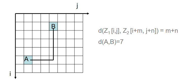
Figure 13: Bloc metric

• metric of edges and centers (checkerboard metric) - the distance between two cells is defined as the minimum number of overcome edges or centers (therefore a diagonal direction of movement is permissible),

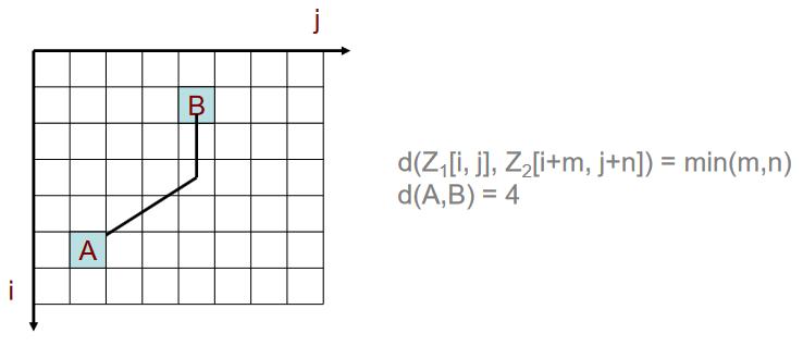
Figure 14: Checkerboard metric

• Euclidean metric - the position of each cell is represented by the position of its center, the distance between cells is then defined as the distance of their centers (Figure 15).

4.5 Data structures used to store raster data - data compression methods

Various data structures are used to store raster data. The simplest is to store raster data in cells, most often in a text file, where there is always three data on a line: row and column index (or coordinates \(i, j\), or \(x, y\)) and the value represented by the cell. This method is the least advantageous in terms of disk space requirements. However, its use is sometimes unavoidable if we need to transfer raster data between two completely incompatible systems.

Another option is to store raster data in a similar array. The main disadvantage of this representation is a significant memory requirement, another disadvantage is that it is necessary to attach to the stored data accompanying data that inform users such as raster dimensions (number of cells per line, number of lines), data resolution in the cell (binary, 8-bit, 24-bit, etc.), the method of storage (rows, columns, segments, or tiles), the shape of the base cell, its real dimensions, or the angle between the axes \(i\) and \(j\) (resp. \(x\) and \(y\)) (in the case of an oblique cell shape), or about the position of the raster in the reference position system and further parameters necessary for the transformation of the raster into this reference system.

Thus, with direct dating of each cell or direct dating of the information layer, it is possible to significantly reduce the volume of stored data by excluding their coordinates or indexes in the system of rows and columns of the raster. Only the contents of individual cells are stored in the data file and their position can be identified based on the data of a special file in which the spatial parameters of the data file are defined (min. And max. Values of coordinates of the examined area. Such a method is used, for example, by the IDRISI system. These parameters do not always form a separate file, they can also be contained in the data file - in its introductory part, the so-called header.

In the simplest case, it is possible to imagine the transcription of a matrix of raster values into a row - a list of cell values by rows or columns (row order), resp. row-prime order - see figure 16. This is also the most commonly used approach (figure 17).

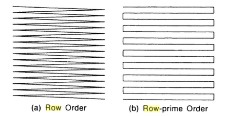
Figure 16: Schema of saving the raster line by line or backwards line by line (source: Bonham-Carter, 2013)

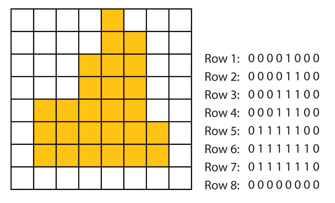
Figure 17: Saving raster line by line (source: https://saylordotorg.github.io/text_essentials-of-geographic-information-systems/s08-01-raster-data-models.html)

It is common for several identical values stored in consecutive cells to be repeated in the order thus created. This is the basis of one of the simplest and most frequently used methods of data compression, the so-called run-length encoding method, in which the original values of data from the cells of the order are replaced by the so-called tupples, which are formed by pairs of numbers: the first indicates the stored value and the second the number of its repetitions in the order (Figure 18).

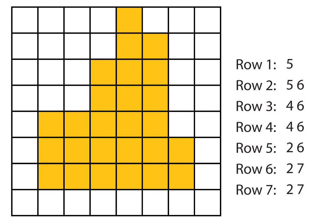
Figure 18: Run-length encoding (zdroj: https://saylordotorg.github.io/text_essentials-of-geographic-information-systems/s08-01-raster-data-models.html)

Other options for determining the order of raster values according to which they will be overwritten from the data matrix to a file:

• Morton order - used for rasters whose dimensions (number of rows and columns) are divisible by 4 and are the same. It is a “zigzag” movement beginning in the lower left corner, creating the shape of an inverted Z in four cells (Figure 19). This movement is repeated at higher hierarchical levels. Morton’s order is used in the length code method as a “space-filling method” when reading raster values. Unlike line-by-line order, elements close to each other in space (area) also become close in order, which is of great importance for some analyzes.

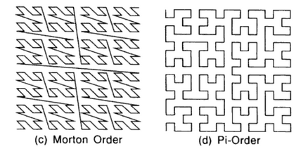
Figure 19: Morton and Peano ordering (source: Bonham-Carter, 2013)

Another interesting feature of Morton’s order (Figure 20) is that if we keep the numbering of rows and columns from 0 and their number is divisible by 2, it is possible to use binary addressing (bit interlaving) to determine the position of the cell in the system of rows and columns based on its position in a series of values created using Morton’s order.

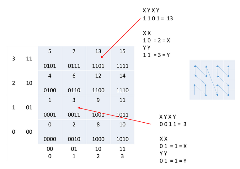
Figure 20: Bináry interleaving (source: https://gistbok.ucgis.org/bok-topics/origins-computing-and-gist-part-2-perspective-role-peripheral-devices)

• Another “space-filling curve” is the Peano curve or Peano order (Pi-Order in Figure 19). Compared to Morton’s order, the changes of direction are rectangular, retaining other advantages.

When directly dating objects, several so-called improved methods of storing raster data can be used:

• Chain codes - define the boundaries of each polygon by encoding the direction (orientation) of the course of the boundary from the specified starting point (Figure 21). The disadvantage of this procedure is the multiple placement of boundary sections common to multiple polygons.

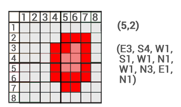
Figure 21: Chain codes (source: https://gisgeography.com/image-compression-encoding/)

• Block codes - indicate the position of the reference points and the size of the square blocks from which the whole object can be created (Figure 22).

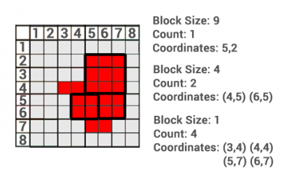
Figure 22: Bloc codes (source: https://gisgeography.com/image-compression-encoding/)

• Run length codes - define the affiliation of raster cells to an object row by row or column, specifying only the beginning and end of a section of cells in a system of rows and columns that have the same value stored (Figure 23). Some authors also refer to this procedure as “standard run-length codes” (Aronof, 1989).

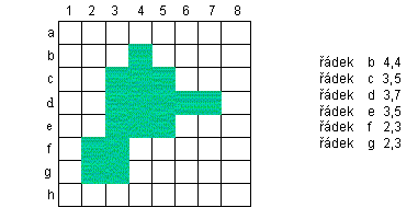
Figure 23: Run length codes

• Quadtree coding - is based on the gradual regular division of the raster into quadrants and subquadrants until either the same value of the observed attribute is the same in the whole quadrant or the smallest possible quadrant dimension (equal to the basic cell dimension) is reached. The goal of this model is to be able to use better spatial resolution to describe the landscape in those places where more detail is needed, without increasing the volume of the database by increasing the pixel size in homogeneous places. Dividing a pixel into quarters always follows when it is found that there is more than one class inside it (Figure 24). From a cartographic point of view, it is a model of a variable scale with a change expressed by the power of two, which is compatible with the conventional Cartesian coordinate system.

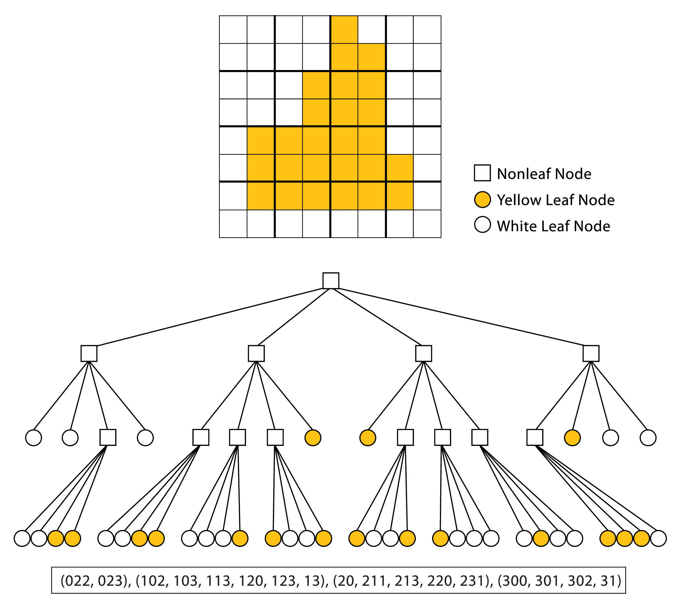
Figure 24: Quadtree (source: https://saylordotorg.github.io/text_essentials-of-geographic-information-systems/s08-01-raster-data-models.html)

A similar procedure can be applied to three-dimensional space, the spatial elements then become cubes and we create the so-called octree.

In practice, a number of data structures have been proposed, enabling the representation of the quadtree in computer memory. The most used are the so-called linear quadtree, in which only end nodes (sheets) are recorded, each node is marked with a special numeric key, from which spatial relationships can be easily derived. This principle is used, for example, in the SPANS software product from Tydac Technologies.

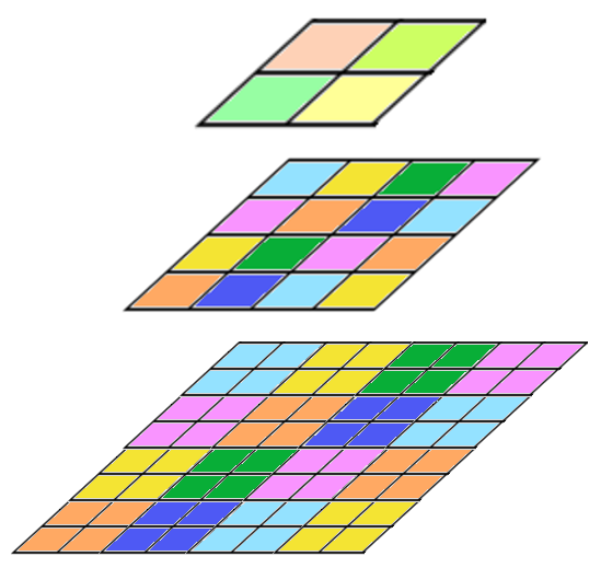
Another hierarchical data structure is the pyramid, which, unlike a quadtree, stores all the cells in a hierarchy, with the value represented in the higher cells usually being determined as the average of the cells one level lower (Figure 25). We proceed by first displaying the raster lying at the highest level, which has the largest dimension of the basic cell and thus the lowest resolution. In this raster we can easily find the area that interests us. Then we switch to the raster, which is one level lower, and perform a more accurate localization of the area of interest. Again, we switch to a raster with a smaller base cell size, which displays the area of interest in much more detail. We repeat these steps until we reach the raster lying at the lowest level of the pyramid, which shows the area of interest in the most detail.

4.6 Evaluation of raster data model

From the point of view of the implementation of individual components of the description of geo-objects, the raster model is the worst off (Rapant, 2002). Most problems arise because in the raster model it is not possible to work directly with individual geo-objects, but only with rasters showing the distribution of properties of geo-objects in the area of interest:

• geometric component is included in this model only implicitly, explicit expression is practically impossible,
• thematic component is realized in the form of individual rasters, showing the distribution of properties in the area of interest,
• time component can be captured only as a sequence of rasters showing the distribution of the same attribute at different time points,
• the reference component can be implemented only to a limited extent, to the extent corresponding to the raster possibilities,
• functional component can be implemented in the form of programs processing rasters.